

73
Transient Heat Conduction
However, if we consider q ˙ = 0, but q "" = −εσ(
r
T 4 − T 4 )
sur , the energy balance
equation can be rewritten as
d(ρVCT) = −hA s (T − T ) − εσA s (T
4
∞
− T
4 )
dt
sur
If let T ∞ = T
2
2
sur , h r = εσ(T + T )(T + T ), the above equation can be
∞
∞
written as
d(T − T ∞ ) (h + h r )A
t
+
s (T T
d
ρVC
− ∞ ) = 0
The solution of the above equation can be obtained by numerical
integration.
4.2 Method of Separation of Variables for 1-D and for
Multidimensional Transient Conduction Problems
4.2.1 1-D Transient Heat Conduction in a Slab
The solution of the 1-D transient conduction problem for a slab (plane wall) is
expected as T(x, t). The separation of variable method used for the 2-D steadystate heat conduction problem can be applied here if we consider T(x, t)
similar to T(x, y). In other words, we separate the temperature T(x, y) into
the product of T(x) · T(y) for the 2-D steady state and T(x, t) into T(x) · T(t)
for the 1-D transient, respectively. Then we can follow the similar procedure
as before in order to solve the 1-D transient problem [1].
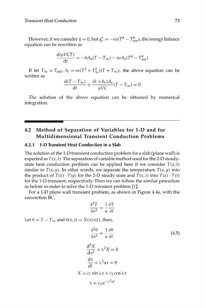
For a 1-D plane wall transient problem, as shown in Figure 4.4a, with the
convection BC,
∂ 2 T
1 ∂T
=
∂x 2
α ∂t
Let θ = T − T ∞ and θ(x, t) = X(x)τ(t), then,
∂ 2 θ
1 ∂θ
=
(4.5)
∂x 2
α ∂t
d 2 X + λ
2 X = 0
dx 2
dτ
2
+ λ ατ = 0
dt
X = c 1 sin λx + c 2 cos λx
−λ 2 αt
τ = c 3 e
Transient Heat Conduction
However, if we consider q ˙ = 0, but q "" = −εσ(
r
T 4 − T 4 )
sur , the energy balance
equation can be rewritten as
d(ρVCT) = −hA s (T − T ) − εσA s (T
4
∞
− T
4 )
dt
sur
If let T ∞ = T
2
2
sur , h r = εσ(T + T )(T + T ), the above equation can be
∞
∞
written as
d(T − T ∞ ) (h + h r )A
t
+
s (T T
d
ρVC
− ∞ ) = 0
The solution of the above equation can be obtained by numerical
integration.
4.2 Method of Separation of Variables for 1-D and for
Multidimensional Transient Conduction Problems
4.2.1 1-D Transient Heat Conduction in a Slab
The solution of the 1-D transient conduction problem for a slab (plane wall) is
expected as T(x, t). The separation of variable method used for the 2-D steadystate heat conduction problem can be applied here if we consider T(x, t)
similar to T(x, y). In other words, we separate the temperature T(x, y) into
the product of T(x) · T(y) for the 2-D steady state and T(x, t) into T(x) · T(t)
for the 1-D transient, respectively. Then we can follow the similar procedure
as before in order to solve the 1-D transient problem [1].
For a 1-D plane wall transient problem, as shown in Figure 4.4a, with the
convection BC,
∂ 2 T
1 ∂T
=
∂x 2
α ∂t
Let θ = T − T ∞ and θ(x, t) = X(x)τ(t), then,
∂ 2 θ
1 ∂θ
=
(4.5)
∂x 2
α ∂t
d 2 X + λ
2 X = 0
dx 2
dτ
2
+ λ ατ = 0
dt
X = c 1 sin λx + c 2 cos λx
−λ 2 αt
τ = c 3 e