3.4.2 Nonhomogeneous Heat Conduction Problem
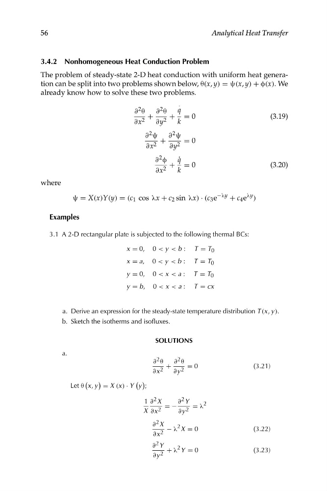
The problem of steady-state 2-D heat conduction with uniform heat generation can be split into two problems shown below, θ(x, y) = ψ(x, y) + φ(x). We
already know how to solve these two problems.
·
∂ 2 θ
∂ 2 θ
q
+
+ = 0
(3.19)
∂x 2
∂y 2
k
∂ 2 ψ ∂ 2 ψ
+
= 0
∂x 2
∂y 2
∂ 2 φ q ˙
+ = 0
(3.20)
∂x 2
k
where
−
λy
ψ = X(x)Y(y) = (c 1 cos λx + c 2 sin λx) · (c 3 e
λy
+ c 4 e )
Examples
3.1 A 2-D rectangular plate is subjected to the following thermal BCs:
x = 0, 0 < y < b : T = T 0
x = a, 0 < y < b : T = T 0
y = 0, 0 < x < a : T = T 0
y = b, 0 < x < a : T = cx
a. Derive an expression for the steady-state temperature distribution T (x, y ).
b. Sketch the isotherms and isofluxes.
SOLUTIONS
a.
∂ 2 θ
∂ 2 θ
+
= 0
(3.21)
∂x 2
∂y 2
(
)
( )
Let θ x, y = X (x) · Y y ;
1 ∂ 2 X
∂ 2 Y
2
= −
= λ
X ∂x 2
∂y 2
∂ 2 X − λ 2 X = 0
(3.22)
∂x 2
∂ 2 Y + λ 2 Y = 0
(3.23)
∂y 2
56
Analytical Heat Transfer