

�
�
50
Analytical Heat Transfer
T 1
T 1
T 1
a
b
"
s
q
∂y
= −k
= given
x
y
θ = T−T 1
θ = 0
θ = 0
θ = 0
∂θ
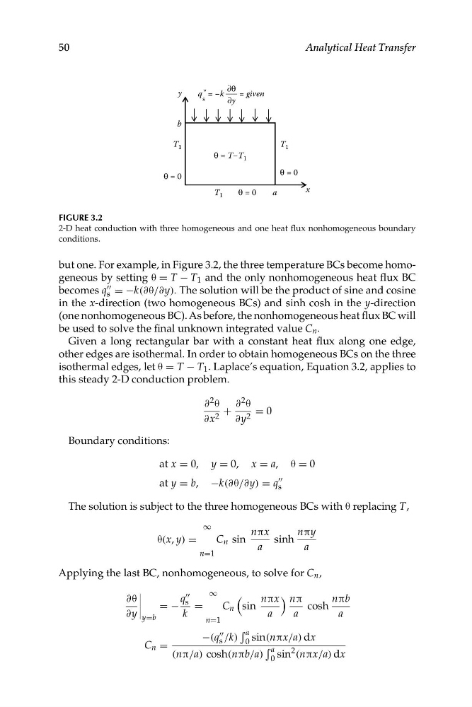
FIGURE 3.2
2-D heat conduction with three homogeneous and one heat flux nonhomogeneous boundary
conditions.
but one. For example, in Figure 3.2, the three temperature BCs become homogeneous by setting θ = T − T 1 and the only nonhomogeneous heat flux BC
""
becomes q = −k(∂θ/∂y). The solution will be the product of sine and cosine
s
in the x-direction (two homogeneous BCs) and sinh cosh in the y-direction
(one nonhomogeneous BC). As before, the nonhomogeneous heat flux BC will
be used to solve the final unknown integrated value C n .
Given a long rectangular bar with a constant heat flux along one edge,
other edges are isothermal. In order to obtain homogeneous BCs on the three
isothermal edges, let θ = T − T 1 . Laplace’s equation, Equation 3.2, applies to
this steady 2-D conduction problem.
∂ 2 θ
∂ 2 θ
+
= 0
∂x 2
∂y 2
Boundary conditions:
at x = 0, y = 0, x = a, θ = 0
""
at y = b, −k(∂θ/∂y) = q s
The solution is subject to the three homogeneous BCs with θ replacing T,
∞
nπx
nπy
θ(x, y) =
C n sin
sinh
a
a
n=1
Applying the last BC, nonhomogeneous, to solve for C n ,
�
∞
""
(
)
∂θ �
�
q s
nπx nπ
nπb
= − =
C n sin
cosh
∂y
k
a
a
a
y=b
n=1
a
""
−(q /k) 0 sin(nπx/a) dx
s
C n =
� a
(nπ/a) cosh(nπb/a) 0 sin
2 (nπx/a) dx
�
50
Analytical Heat Transfer
T 1
T 1
T 1
a
b
"
s
q
∂y
= −k
= given
x
y
θ = T−T 1
θ = 0
θ = 0
θ = 0
∂θ
FIGURE 3.2
2-D heat conduction with three homogeneous and one heat flux nonhomogeneous boundary
conditions.
but one. For example, in Figure 3.2, the three temperature BCs become homogeneous by setting θ = T − T 1 and the only nonhomogeneous heat flux BC
""
becomes q = −k(∂θ/∂y). The solution will be the product of sine and cosine
s
in the x-direction (two homogeneous BCs) and sinh cosh in the y-direction
(one nonhomogeneous BC). As before, the nonhomogeneous heat flux BC will
be used to solve the final unknown integrated value C n .
Given a long rectangular bar with a constant heat flux along one edge,
other edges are isothermal. In order to obtain homogeneous BCs on the three
isothermal edges, let θ = T − T 1 . Laplace’s equation, Equation 3.2, applies to
this steady 2-D conduction problem.
∂ 2 θ
∂ 2 θ
+
= 0
∂x 2
∂y 2
Boundary conditions:
at x = 0, y = 0, x = a, θ = 0
""
at y = b, −k(∂θ/∂y) = q s
The solution is subject to the three homogeneous BCs with θ replacing T,
∞
nπx
nπy
θ(x, y) =
C n sin
sinh
a
a
n=1
Applying the last BC, nonhomogeneous, to solve for C n ,
�
∞
""
(
)
∂θ �
�
q s
nπx nπ
nπb
= − =
C n sin
cosh
∂y
k
a
a
a
y=b
n=1
a
""
−(q /k) 0 sin(nπx/a) dx
s
C n =
� a
(nπ/a) cosh(nπb/a) 0 sin
2 (nπx/a) dx