

�
�
�
�
�
�
�
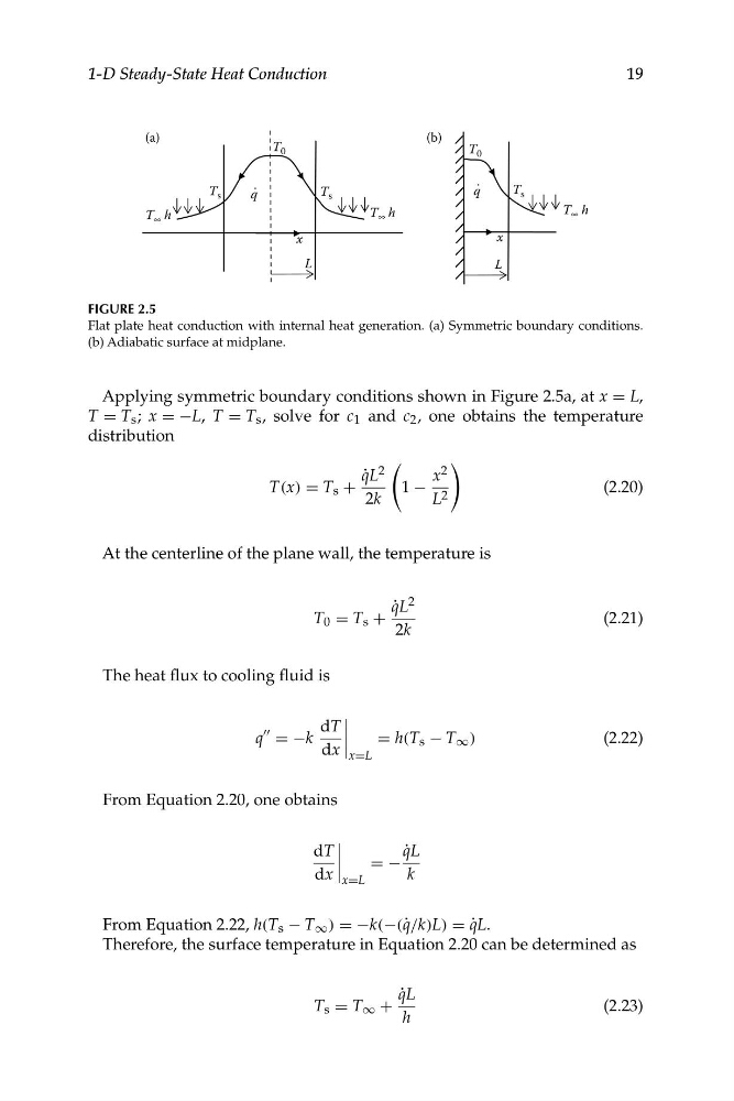
Applying symmetric boundary conditions shown in Figure 2.5a, at x = L,
T = T s ; x = −L, T = T s , solve for c 1 and c 2 , one obtains the temperature
distribution
2
˙
x
qL 2
T(x) = T s +
1 −
(2.20)
2k
L 2
At the centerline of the plane wall, the temperature is
˙
qL 2
T 0 = T s +
(2.21)
2k
The heat flux to cooling fluid is
dT �
q
""
= −k
�
= h(T s − T ∞ )
(2.22)
dx x=L
From Equation 2.20, one obtains
dT �
˙
qL
= −
dx
k
x=L
From Equation 2.22, h(T s − T ∞ ) = −k(−(q ˙/k)L) = ˙
qL.
Therefore, the surface temperature in Equation 2.20 can be determined as
˙
qL
T s = T ∞ +
(2.23)
h
19
1-D Steady-State Heat Conduction
T ∞ h
T 0
T 0
L
T s
x
T ∞ h
T s
T s
T ∞ h
L
x
(a)
(b)
q
.
q
.
FIGURE 2.5
Flat plate heat conduction with internal heat generation. (a) Symmetric boundary conditions.
(b) Adiabatic surface at midplane.
�
�
�
�
�
�
Applying symmetric boundary conditions shown in Figure 2.5a, at x = L,
T = T s ; x = −L, T = T s , solve for c 1 and c 2 , one obtains the temperature
distribution
2
˙
x
qL 2
T(x) = T s +
1 −
(2.20)
2k
L 2
At the centerline of the plane wall, the temperature is
˙
qL 2
T 0 = T s +
(2.21)
2k
The heat flux to cooling fluid is
dT �
q
""
= −k
�
= h(T s − T ∞ )
(2.22)
dx x=L
From Equation 2.20, one obtains
dT �
˙
qL
= −
dx
k
x=L
From Equation 2.22, h(T s − T ∞ ) = −k(−(q ˙/k)L) = ˙
qL.
Therefore, the surface temperature in Equation 2.20 can be determined as
˙
qL
T s = T ∞ +
(2.23)
h
19
1-D Steady-State Heat Conduction
T ∞ h
T 0
T 0
L
T s
x
T ∞ h
T s
T s
T ∞ h
L
x
(a)
(b)
q
.
q
.
FIGURE 2.5
Flat plate heat conduction with internal heat generation. (a) Symmetric boundary conditions.
(b) Adiabatic surface at midplane.