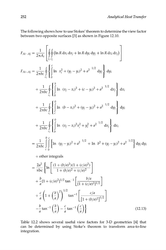
�
�
�
�
�
�
�
�
�
�
�
�
� �
� �
� �
�
� �
� � {
�
� �
�
�
�
�
�
�
The following shows how to use Stokes’ theorem to determine the view factor
between two opposite surfaces [3] as shown in Figure 12.10.
⎡
⎤
1
(
)
ln R dx i dx j + ln R dy i dy j + ln R dz i dz j
F Ai−Aj
⎢
⎥
⎦
=
⎣
2πA i
c i c j
⎧
⎫
c
1
⎨
⎩
2
2
ln x i + (y j − y i )
2
+ a
1/2
⎬
dy j dy i
F Ai−Aj = 2πbc
⎭
c i 0
⎧
⎫
b
1
+ 2πbc
⎨
⎩
2
ln (x j − x i )
2
+ (c − y i )
2
+ a
1/2
⎬
dx j dx i
⎭
c i 0
⎧
⎫
0
1
+ 2πbc
⎨
⎩
�
c
2
ln (b − x i )
2
+ (y j − y i )
2
+ a
1/2
⎬
dy j dy i
⎭
c i
⎧
⎫
0
1
2πbc
1/2
⎨
⎩
⎬
2 2
2
2
ln (x j − x i ) x + y + a
dx j dx i
+
i
i
⎭
c i b
0 c
1/2
1/2
2
2
ln (y j − y i )
2
+ a
+ ln b
2
+ (y j − y i )
2
+ a
1
= 2πbc
dy j dy i
c 0
+ other integrals
2a
2
(1 + (b/a) 2 )(1 + (c/a) 2 )
=
ln
πbc
1 + (b/a) 2 + (c/a) 2
b
b/a
+ [1 + (c/a)
2
]
1/2 tan
−1
a
[1 + (c/a) 2 ] 1/2
� � 2
� 1/2
c
b
c/a
+
1 +
tan
−1
a
a
[
1 + (b/a) 2
] 1/2
� �
� ��
b
b
c
c
− tan
−1
− tan
−1
(12.13)
a
a
a
a
Table 12.2 shows several useful view factors for 3-D geometries [4] that
can be determined by using Stoke’s theorem to transform area-to-line
integration.
252
Analytical Heat Transfer