

11
Heat Conduction Equations
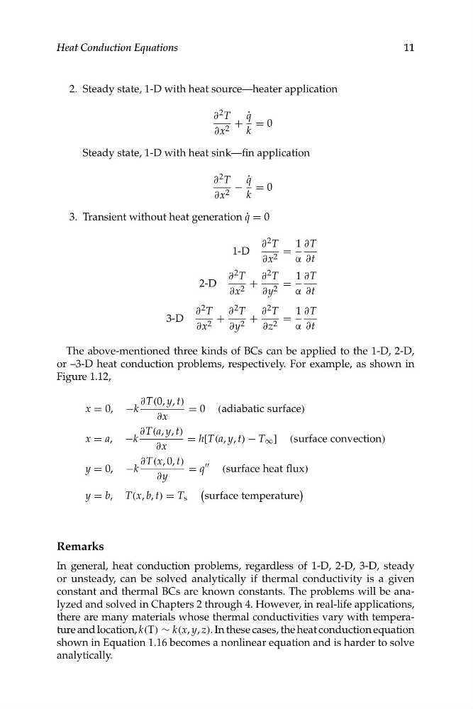
2. Steady state, 1-D with heat source—heater application
∂ 2 T
q ˙
+ = 0
∂x 2
k
Steady state, 1-D with heat sink—fin application
∂ 2 T
q ˙
− = 0
∂x 2
k
3. Transient without heat generation q ˙ = 0
∂ 2 T
1 ∂T
1-D
=
∂x 2
α ∂t
∂ 2 T
∂ 2 T
1 ∂T
2-D
+
=
∂x 2
∂y 2
α ∂t
∂ 2 T
∂ 2 T
∂ 2 T
1 ∂T
3-D
+
+
=
∂x 2
∂y 2
∂z 2
α ∂t
The above-mentioned three kinds of BCs can be applied to the 1-D, 2-D,
or –3-D heat conduction problems, respectively. For example, as shown in
Figure 1.12,
∂T(0, y, t)
x = 0, −k
= 0 (adiabatic surface)
∂x
∂T(a, y, t)
x = a, −k
= h[T(a, y, t) − T ∞ ] (surface convection)
∂x
∂T(x, 0, t)
""
y = 0, −k
= q
(surface heat flux)
∂y
(
)
y = b, T(x, b, t) = T s
surface temperature
Remarks
In general, heat conduction problems, regardless of 1-D, 2-D, 3-D, steady
or unsteady, can be solved analytically if thermal conductivity is a given
constant and thermal BCs are known constants. The problems will be analyzed and solved in Chapters 2 through 4. However, in real-life applications,
there are many materials whose thermal conductivities vary with temperature and location, k(T) ∼ k(x, y, z). In these cases, the heat conduction equation
shown in Equation 1.16 becomes a nonlinear equation and is harder to solve
analytically.
Heat Conduction Equations
2. Steady state, 1-D with heat source—heater application
∂ 2 T
q ˙
+ = 0
∂x 2
k
Steady state, 1-D with heat sink—fin application
∂ 2 T
q ˙
− = 0
∂x 2
k
3. Transient without heat generation q ˙ = 0
∂ 2 T
1 ∂T
1-D
=
∂x 2
α ∂t
∂ 2 T
∂ 2 T
1 ∂T
2-D
+
=
∂x 2
∂y 2
α ∂t
∂ 2 T
∂ 2 T
∂ 2 T
1 ∂T
3-D
+
+
=
∂x 2
∂y 2
∂z 2
α ∂t
The above-mentioned three kinds of BCs can be applied to the 1-D, 2-D,
or –3-D heat conduction problems, respectively. For example, as shown in
Figure 1.12,
∂T(0, y, t)
x = 0, −k
= 0 (adiabatic surface)
∂x
∂T(a, y, t)
x = a, −k
= h[T(a, y, t) − T ∞ ] (surface convection)
∂x
∂T(x, 0, t)
""
y = 0, −k
= q
(surface heat flux)
∂y
(
)
y = b, T(x, b, t) = T s
surface temperature
Remarks
In general, heat conduction problems, regardless of 1-D, 2-D, 3-D, steady
or unsteady, can be solved analytically if thermal conductivity is a given
constant and thermal BCs are known constants. The problems will be analyzed and solved in Chapters 2 through 4. However, in real-life applications,
there are many materials whose thermal conductivities vary with temperature and location, k(T) ∼ k(x, y, z). In these cases, the heat conduction equation
shown in Equation 1.16 becomes a nonlinear equation and is harder to solve
analytically.