

�
�
�
�
�
and
+
+
u = y
(10.35)
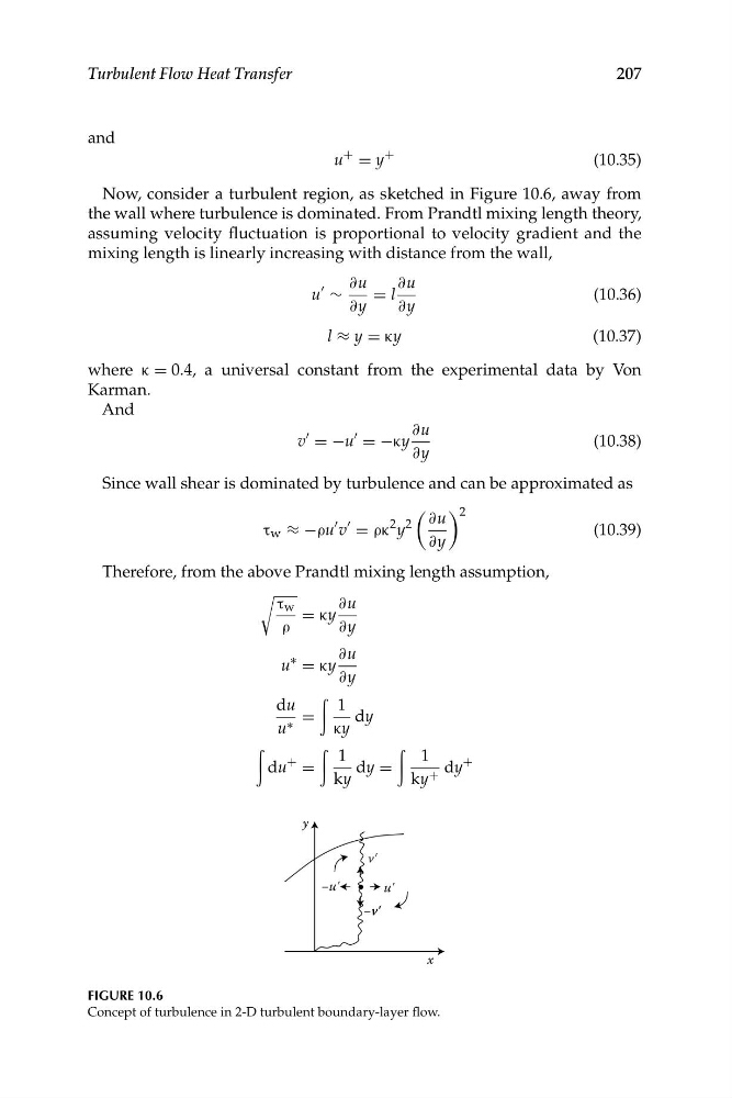
Now, consider a turbulent region, as sketched in Figure 10.6, away from
the wall where turbulence is dominated. From Prandtl mixing length theory,
assuming velocity fluctuation is proportional to velocity gradient and the
mixing length is linearly increasing with distance from the wall,
∂u
∂u
u
"
∼
= l
(10.36)
∂y
∂y
l ≈ y = κy
(10.37)
where κ = 0.4, a universal constant from the experimental data by Von
Karman.
And
∂u
v
"
= −u
"
= −κy
(10.38)
∂y
Since wall shear is dominated by turbulence and can be approximated as
� � 2
∂u
" "
2 2
τ w ≈ −ρu v = ρκ y
(10.39)
∂y
Therefore, from the above Prandtl mixing length assumption,
τ w
∂u
= κy
ρ
∂y
∂u
∗
u = κy
∂y
du
1
=
dy
u ∗
κy
+
1
1
+
du =
dy =
dy
ky
ky +
207
Turbulent Flow Heat Transfer
u'
v'
v'
−v'
−u'
y
x
FIGURE 10.6
Concept of turbulence in 2-D turbulent boundary-layer flow.
�
�
�
�
and
+
+
u = y
(10.35)
Now, consider a turbulent region, as sketched in Figure 10.6, away from
the wall where turbulence is dominated. From Prandtl mixing length theory,
assuming velocity fluctuation is proportional to velocity gradient and the
mixing length is linearly increasing with distance from the wall,
∂u
∂u
u
"
∼
= l
(10.36)
∂y
∂y
l ≈ y = κy
(10.37)
where κ = 0.4, a universal constant from the experimental data by Von
Karman.
And
∂u
v
"
= −u
"
= −κy
(10.38)
∂y
Since wall shear is dominated by turbulence and can be approximated as
� � 2
∂u
" "
2 2
τ w ≈ −ρu v = ρκ y
(10.39)
∂y
Therefore, from the above Prandtl mixing length assumption,
τ w
∂u
= κy
ρ
∂y
∂u
∗
u = κy
∂y
du
1
=
dy
u ∗
κy
+
1
1
+
du =
dy =
dy
ky
ky +
207
Turbulent Flow Heat Transfer
u'
v'
v'
−v'
−u'
y
x
FIGURE 10.6
Concept of turbulence in 2-D turbulent boundary-layer flow.