

Therefore,
� η
� η � η − 0 1/2( f dη) dη dη
0 e
f =
0
� η
(7.20)
∞ − 0 1/2(f dη) dη
e
0
�
�
145
External Forced Convection
�
For example, use of the trapezoidal rule for the numerical integrations:
Choose η max = 5 = Δη · N, when N = 50 (the number of integration steps),
Δη = 0.1
Let η i+1 = η i + Δη for i = 0, 1, 2, . . . , with η o = 0
Initial guess f i = η i � η i
� η i
� η i
� η i
−
f dη
� η i −
� η i � η i −
Calculate
f dη, e 0
,
e 0 f dη dη, and
e 0 f dη dη dη
0
(
0
)
0 0
� η i
� η max − f dη dη
""
Calculate C 1 = 1/
e 0
, f i , f "
0
i , f i
� 1 − f new /f old �
Check convergence
i
i
< ε?, for i = 0, 1, 2, . . . , N. If not, go back
again.
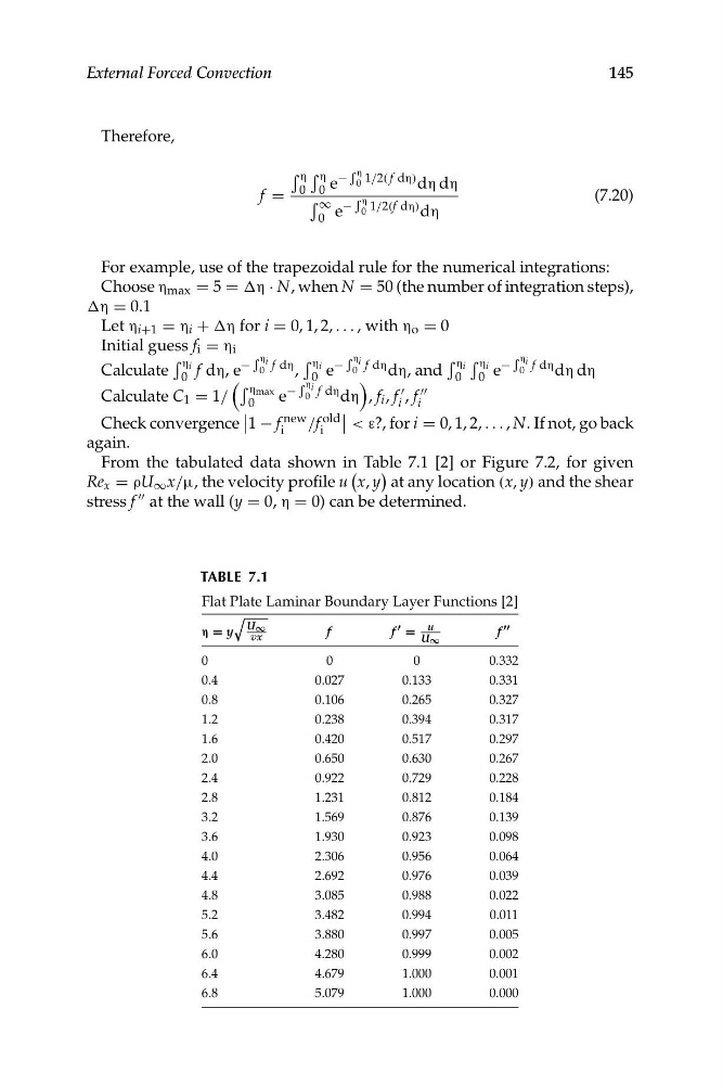
From the tabulated data shown in Table 7.1 [2] or Figure 7.2, for given
( )
Re x = ρU ∞ x/μ, the velocity profile u x, y at any location (x, y) and the shear
stress f "" at the wall (y = 0, η = 0) can be determined.
TABLE 7.1
Flat Plate Laminar Boundary Layer Functions [2]
[
U ∞
u
f ""
η = y
f
f " =
vx
U ∞
0
0
0
0.332
0.4
0.027
0.133
0.331
0.8
0.106
0.265
0.327
1.2
0.238
0.394
0.317
1.6
0.420
0.517
0.297
2.0
0.650
0.630
0.267
2.4
0.922
0.729
0.228
2.8
1.231
0.812
0.184
3.2
1.569
0.876
0.139
3.6
1.930
0.923
0.098
4.0
2.306
0.956
0.064
4.4
2.692
0.976
0.039
4.8
3.085
0.988
0.022
5.2
3.482
0.994
0.011
5.6
3.880
0.997
0.005
6.0
4.280
0.999
0.002
6.4
4.679
1.000
0.001
6.8
5.079
1.000
0.000
� η
� η � η − 0 1/2( f dη) dη dη
0 e
f =
0
� η
(7.20)
∞ − 0 1/2(f dη) dη
e
0
�
�
145
External Forced Convection
�
For example, use of the trapezoidal rule for the numerical integrations:
Choose η max = 5 = Δη · N, when N = 50 (the number of integration steps),
Δη = 0.1
Let η i+1 = η i + Δη for i = 0, 1, 2, . . . , with η o = 0
Initial guess f i = η i � η i
� η i
� η i
� η i
−
f dη
� η i −
� η i � η i −
Calculate
f dη, e 0
,
e 0 f dη dη, and
e 0 f dη dη dη
0
(
0
)
0 0
� η i
� η max − f dη dη
""
Calculate C 1 = 1/
e 0
, f i , f "
0
i , f i
� 1 − f new /f old �
Check convergence
i
i
< ε?, for i = 0, 1, 2, . . . , N. If not, go back
again.
From the tabulated data shown in Table 7.1 [2] or Figure 7.2, for given
( )
Re x = ρU ∞ x/μ, the velocity profile u x, y at any location (x, y) and the shear
stress f "" at the wall (y = 0, η = 0) can be determined.
TABLE 7.1
Flat Plate Laminar Boundary Layer Functions [2]
[
U ∞
u
f ""
η = y
f
f " =
vx
U ∞
0
0
0
0.332
0.4
0.027
0.133
0.331
0.8
0.106
0.265
0.327
1.2
0.238
0.394
0.317
1.6
0.420
0.517
0.297
2.0
0.650
0.630
0.267
2.4
0.922
0.729
0.228
2.8
1.231
0.812
0.184
3.2
1.569
0.876
0.139
3.6
1.930
0.923
0.098
4.0
2.306
0.956
0.064
4.4
2.692
0.976
0.039
4.8
3.085
0.988
0.022
5.2
3.482
0.994
0.011
5.6
3.880
0.997
0.005
6.0
4.280
0.999
0.002
6.4
4.679
1.000
0.001
6.8
5.079
1.000
0.000