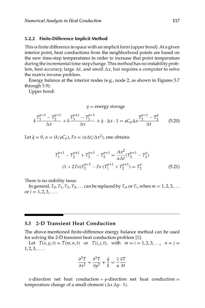
q = energy storage
T
p+1 − T
p+1
T
p+1 − T
p+1
T
p+1 − T
p

1
2
3
2
2
2

k
+ k
+ q ˙ · Δx · 1 = ρC p Δx
(5.20)
Δx
Δx
Δt
Let q ˙ = 0, α = (k/ρC p ), Fo = (αΔt/Δx 2 ), one obtains
2
Δx
− T
p
T
p+1 − T
p+1 + T
p+1 − T
p+1
(T
p+1
=
1
2
3
2
2
2 )
αΔt
+ T
p+1 = T
p
(1 + 2 Fo)T
p+1 − Fo (T
p+1
)
(5.21)
2
1
2
2
Numerical Analysis in Heat Conduction
117
5.2.2 Finite-Difference Implicit Method
This is finite difference in space with an implicit form (upper bond). At a given
interior point, heat conductions from the neighborhood points are based on
the new time-step temperatures in order to increase that point temperature
during the incremental time-step change. This method has no instability problem, best accuracy, large Δt, and small Δx, but requires a computer to solve
the matrix inverse problem.
Energy balance at the interior nodes (e.g., node 2, as shown in Figures 5.7
through 5.9):
Upper bond:
There is no stability issue.
In general, T 0 , T 1 , T 2 , T 3 , . . . can be replaced by T m or T i , when m = 1, 2, 3, . . .
or i = 1, 2, 3, . . . .
5.3 2-D Transient Heat Conduction
The above-mentioned finite-difference energy balance method can be used
for solving the 2-D transient heat conduction problem [1].
Let T(x, y, t) = T(m, n, t) or T(i, j, t), with m = i = 1, 2, 3, . . ., n = j =
1, 2, 3, . . . .
∂ 2 T
∂ 2 T
q ˙
1 ∂T
+
+ =
∂x 2
∂y 2
k
α ∂t
x-direction net heat conduction + y-direction net heat conduction =
temperature change of a small element (Δx Δy · 1).