

T s
y
x
0
1
2
3
4
1
2
Δx
p
T 3
p
p step
T 4
p
T 1
T i
p
T 2
T 2
p+1
T 3
p+1
T 4
T 1
p + 1 step
p+1
p+1
Δx
�
�
115
Numerical Analysis in Heat Conduction
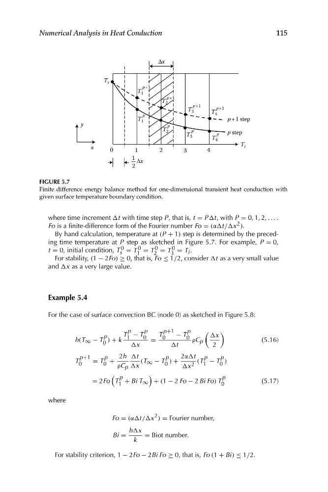
FIGURE 5.7
Finite difference energy balance method for one-dimensional transient heat conduction with
given surface temperature boundary condition.
where time increment Δt with time step P , that is, t = P Δt , with P = 0, 1, 2, . . . .
Fo is a finite-difference form of the Fourier number Fo = (αΔt /Δx 2 ).
By hand calculation, temperature at (P + 1) step is determined by the preceding time temperature at P step as sketched in Figure 5.7. For example, P = 0,
t = 0, initial condition, T 0 = T 0 = T 0 = T 0 = T i .
s
1
2
3
For stability, (1 − 2Fo) ≥ 0, that is, Fo ≤ 1/2, consider Δt as a very small value
and Δx as a very large value.
Example 5.4
For the case of surface convection BC (node 0) as sketched in Figure 5.8:
T
p
T
p+1
1 − T
p
− T
p
Δx
0
0
0
h(T ∞ − T 0
p ) + k
=
ρC p
(5.16)
Δx
Δt
2
2h Δt
2αΔt
0
0 +
0 ) +
0 )
T
p+1 = T
p
(T ∞ − T
p
(T 1
p − T
p
ρC p Δx
Δx 2
(
)
= 2Fo T 1
p + Bi T ∞ + (1 − 2 Fo − 2 Bi Fo) T
p
(5.17)
0
where
Fo = (αΔt /Δx 2 ) = Fourier number,
hΔx
Bi =
= Biot number.
k
For stability criterion, 1 − 2Fo − 2Bi Fo ≥ 0, that is, Fo (1 + Bi) ≤ 1/2.
y
x
0
1
2
3
4
1
2
Δx
p
T 3
p
p step
T 4
p
T 1
T i
p
T 2
T 2
p+1
T 3
p+1
T 4
T 1
p + 1 step
p+1
p+1
Δx
�
�
115
Numerical Analysis in Heat Conduction
FIGURE 5.7
Finite difference energy balance method for one-dimensional transient heat conduction with
given surface temperature boundary condition.
where time increment Δt with time step P , that is, t = P Δt , with P = 0, 1, 2, . . . .
Fo is a finite-difference form of the Fourier number Fo = (αΔt /Δx 2 ).
By hand calculation, temperature at (P + 1) step is determined by the preceding time temperature at P step as sketched in Figure 5.7. For example, P = 0,
t = 0, initial condition, T 0 = T 0 = T 0 = T 0 = T i .
s
1
2
3
For stability, (1 − 2Fo) ≥ 0, that is, Fo ≤ 1/2, consider Δt as a very small value
and Δx as a very large value.
Example 5.4
For the case of surface convection BC (node 0) as sketched in Figure 5.8:
T
p
T
p+1
1 − T
p
− T
p
Δx
0
0
0
h(T ∞ − T 0
p ) + k
=
ρC p
(5.16)
Δx
Δt
2
2h Δt
2αΔt
0
0 +
0 ) +
0 )
T
p+1 = T
p
(T ∞ − T
p
(T 1
p − T
p
ρC p Δx
Δx 2
(
)
= 2Fo T 1
p + Bi T ∞ + (1 − 2 Fo − 2 Bi Fo) T
p
(5.17)
0
where
Fo = (αΔt /Δx 2 ) = Fourier number,
hΔx
Bi =
= Biot number.
k
For stability criterion, 1 − 2Fo − 2Bi Fo ≥ 0, that is, Fo (1 + Bi) ≤ 1/2.