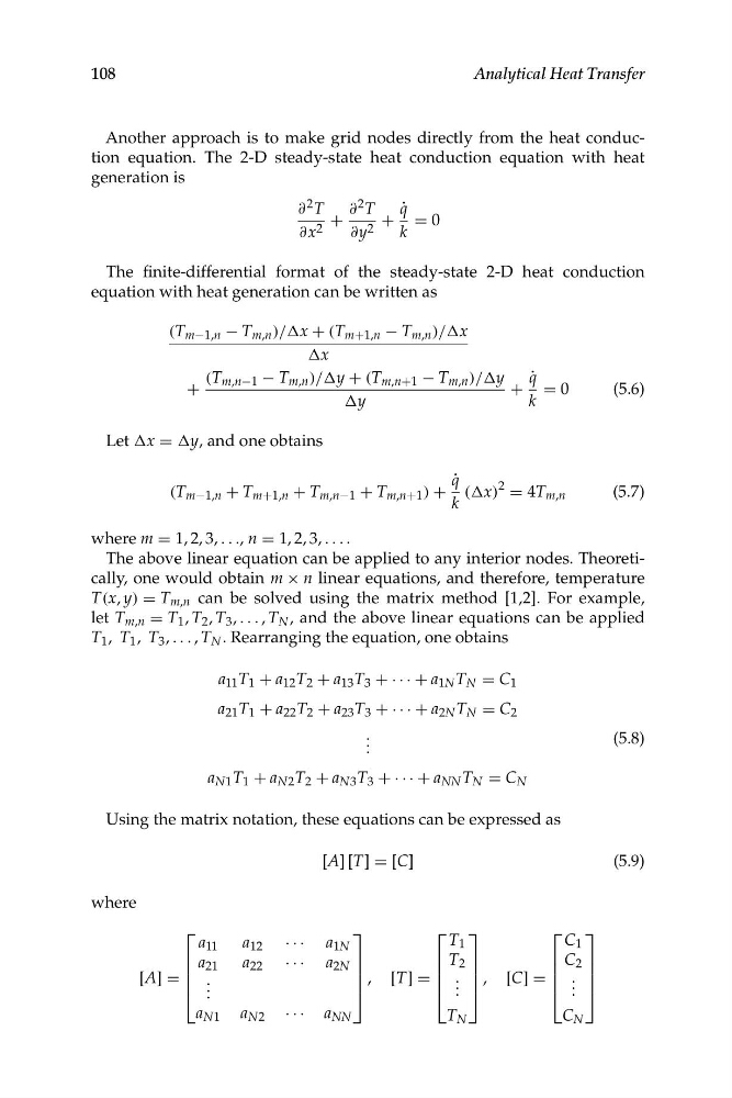
Another approach is to make grid nodes directly from the heat conduction equation. The 2-D steady-state heat conduction equation with heat
generation is
∂ 2 T
∂ 2 T
q ˙
+
+ = 0
∂x 2
∂y 2
k
The finite-differential format of the steady-state 2-D heat conduction
equation with heat generation can be written as
(T m−1,n − T m,n )/Δx + (T m+1,n − T m,n )/Δx
Δx
(T m,n−1 − T m,n )/Δy + (T m,n+1 − T m,n )/Δy q ˙
+
+ = 0
(5.6)
Δy
k
Let Δx = Δy, and one obtains
q ˙
(T m−1,n + T m+1,n + T m,n−1 + T m,n+1 ) + (Δx)
2
= 4T m,n
(5.7)
k
where m = 1, 2, 3, . . ., n = 1, 2, 3, . . . .
The above linear equation can be applied to any interior nodes. Theoretically, one would obtain m × n linear equations, and therefore, temperature
T(x, y) = T m,n can be solved using the matrix method [1,2]. For example,
let T m,n = T 1 , T 2 , T 3 , . . . , T N , and the above linear equations can be applied
T 1 , T 1 , T 3 , . . . , T N . Rearranging the equation, one obtains
a 11 T 1 + a 12 T 2 + a 13 T 3 + · · · + a 1N T N = C 1
a 21 T 1 + a 22 T 2 + a 23 T 3 + · · · + a 2N T N = C 2
. .
(5.8)
.
a N1 T 1 + a N2 T 2 + a N3 T 3 + · · · + a NN T N = C N
Using the matrix notation, these equations can be expressed as
[A] [T] = [C]
(5.9)
where
[A] =
⎡
⎢
⎢
⎢
⎣
a 11
a 21
. . .
a 12
a 22
· · ·
· · ·
a 1N
a 2N
⎤
⎥
⎥
⎥
⎦
, [T] =
⎡
⎢
⎢
⎢
⎣
T 1
T 2
. . .
⎤
⎥
⎥
⎥
⎦
, [C] =
⎡
⎢
⎢
⎢
⎣
C 1
C 2
. . .
⎤
⎥
⎥
⎥
⎦
a N1 a N2 · · · a NN
T N
C N
108
Analytical Heat Transfer