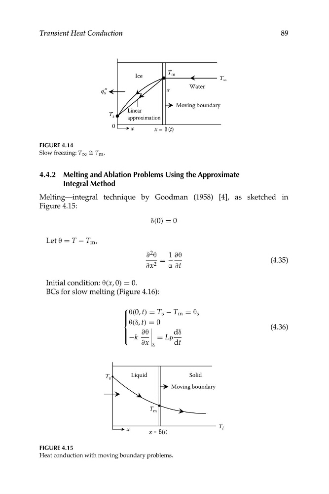
Melting—integral technique by Goodman (1958) [4], as sketched in
Figure 4.15:
δ(0) = 0
Let θ = T − T m ,
∂ 2 θ
∂x 2 =
1
α
∂θ
∂t
(4.35)
Initial condition: θ(x, 0) = 0.
BCs for slow melting (Figure 4.16):
⎧
⎪ ⎪ ⎨
⎪ ⎪ ⎩
θ(0, t) = T s − T m = θ s
θ(δ, t) = 0
−k
∂θ
∂x
�
�
�
�
δ
= Lρ
dδ
dt
(4.36)
89
Transient Heat Conduction
x
Moving boundary
Water
Ice
0
x
Linear
approximation
δ
T s
T ∞
q s ″
T m
x = (t)
FIGURE 4.14
Slow freezing: T ∞ ∼ = T m .
4.4.2 Melting and Ablation Problems Using the Approximate
Integral Method
x
Moving boundary
δ
Solid
Liquid
T s
T i
x = (t)
T m
FIGURE 4.15
Heat conduction with moving boundary problems.