

100
Electromagnetic Fields in Biological Systems
with
A = (E 0 − B) b 3 + C
(2.20b)
B = 3ε E E 0 b 3 (ε I + 2ε M )/[b 3 (ε M + 2ε E )(ε I + 2ε M ) + 2a 3 (ε M − ε E )(ε I − ε M )] (2.20c)
C = 3ε E E 0 a 3 b 3 (ε I − ε M )/[b 3 (ε M + 2ε E )(ε I + 2ε M ) + 2a 3 (ε M − ε E )(ε I − ε M )] (2.20d)
The dielectric constants ε I , ε E , and ε M for the intracellular, extracellular regions, and
the membrane, respectively, are given by the following general expression:
ε k = ε ∞k + [ε k (0) − ε ∞k ]/[1 + jωτ k ] − jσ 0k /(ωε 0 )
(2.20e)
with k representing one of the three regions. Clearly, for a very short pulse (say having
subnanosecond duration), a large number of frequency components would contribute,
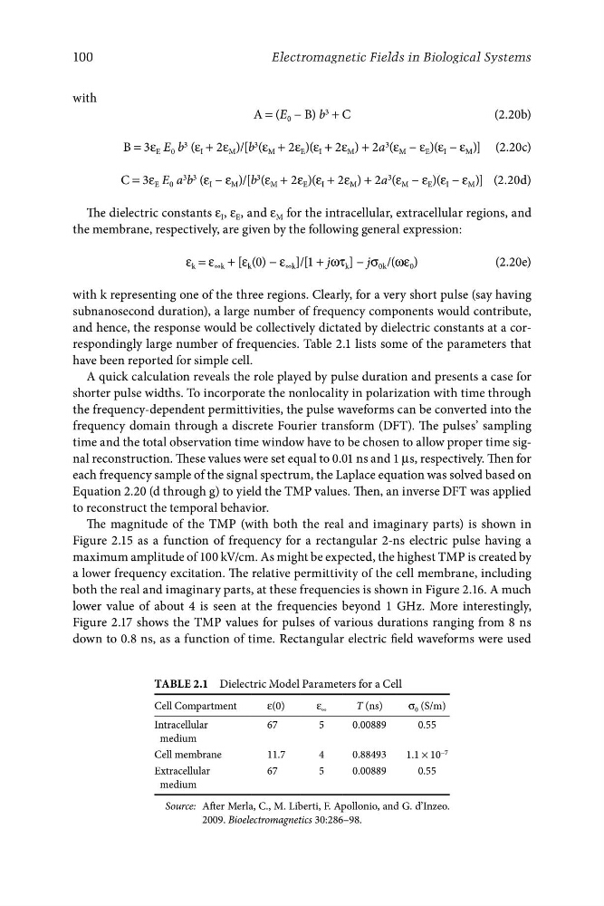
and hence, the response would be collectively dictated by dielectric constants at a correspondingly large number of frequencies. Table 2.1 lists some of the parameters that
have been reported for simple cell.
A quick calculation reveals the role played by pulse duration and presents a case for
shorter pulse widths. To incorporate the nonlocality in polarization with time through
the frequency-dependent permittivities, the pulse waveforms can be converted into the
frequency domain through a discrete Fourier transform (DFT). The pulses’ sampling
time and the total observation time window have to be chosen to allow proper time signal reconstruction. These values were set equal to 0.01 ns and 1 μs, respectively. Then for
each frequency sample of the signal spectrum, the Laplace equation was solved based on
Equation 2.20 (d through g) to yield the TMP values. Then, an inverse DFT was applied
to reconstruct the temporal behavior.
The magnitude of the TMP (with both the real and imaginary parts) is shown in
Figure 2.15 as a function of frequency for a rectangular 2-ns electric pulse having a
maximum amplitude of 100 kV/cm. As might be expected, the highest TMP is created by
a lower frequency excitation. The relative permittivity of the cell membrane, including
both the real and imaginary parts, at these frequencies is shown in Figure 2.16. A much
lower value of about 4 is seen at the frequencies beyond 1 GHz. More interestingly,
Figure 2.17 shows the TMP values for pulses of various durations ranging from 8 ns
down to 0.8 ns, as a function of time. Rectangular electric field waveforms were used
Table 2.1 Dielectric Model Parameters for a Cell
Cell Compartment
ε(0)
ε ∞
T (ns)
σ 0 (S/m)
Intracellular
67
5
0.00889
0.55
medium
Cell membrane
11.7
4
0.88493
1.1 × 10 −7
Extracellular
67
5
0.00889
0.55
medium
Source: After Merla, C., M. Liberti, F. Apollonio, and G. d’Inzeo.
2009. Bioelectromagnetics 30:286–98.
Electromagnetic Fields in Biological Systems
with
A = (E 0 − B) b 3 + C
(2.20b)
B = 3ε E E 0 b 3 (ε I + 2ε M )/[b 3 (ε M + 2ε E )(ε I + 2ε M ) + 2a 3 (ε M − ε E )(ε I − ε M )] (2.20c)
C = 3ε E E 0 a 3 b 3 (ε I − ε M )/[b 3 (ε M + 2ε E )(ε I + 2ε M ) + 2a 3 (ε M − ε E )(ε I − ε M )] (2.20d)
The dielectric constants ε I , ε E , and ε M for the intracellular, extracellular regions, and
the membrane, respectively, are given by the following general expression:
ε k = ε ∞k + [ε k (0) − ε ∞k ]/[1 + jωτ k ] − jσ 0k /(ωε 0 )
(2.20e)
with k representing one of the three regions. Clearly, for a very short pulse (say having
subnanosecond duration), a large number of frequency components would contribute,
and hence, the response would be collectively dictated by dielectric constants at a correspondingly large number of frequencies. Table 2.1 lists some of the parameters that
have been reported for simple cell.
A quick calculation reveals the role played by pulse duration and presents a case for
shorter pulse widths. To incorporate the nonlocality in polarization with time through
the frequency-dependent permittivities, the pulse waveforms can be converted into the
frequency domain through a discrete Fourier transform (DFT). The pulses’ sampling
time and the total observation time window have to be chosen to allow proper time signal reconstruction. These values were set equal to 0.01 ns and 1 μs, respectively. Then for
each frequency sample of the signal spectrum, the Laplace equation was solved based on
Equation 2.20 (d through g) to yield the TMP values. Then, an inverse DFT was applied
to reconstruct the temporal behavior.
The magnitude of the TMP (with both the real and imaginary parts) is shown in
Figure 2.15 as a function of frequency for a rectangular 2-ns electric pulse having a
maximum amplitude of 100 kV/cm. As might be expected, the highest TMP is created by
a lower frequency excitation. The relative permittivity of the cell membrane, including
both the real and imaginary parts, at these frequencies is shown in Figure 2.16. A much
lower value of about 4 is seen at the frequencies beyond 1 GHz. More interestingly,
Figure 2.17 shows the TMP values for pulses of various durations ranging from 8 ns
down to 0.8 ns, as a function of time. Rectangular electric field waveforms were used
Table 2.1 Dielectric Model Parameters for a Cell
Cell Compartment
ε(0)
ε ∞
T (ns)
σ 0 (S/m)
Intracellular
67
5
0.00889
0.55
medium
Cell membrane
11.7
4
0.88493
1.1 × 10 −7
Extracellular
67
5
0.00889
0.55
medium
Source: After Merla, C., M. Liberti, F. Apollonio, and G. d’Inzeo.
2009. Bioelectromagnetics 30:286–98.