

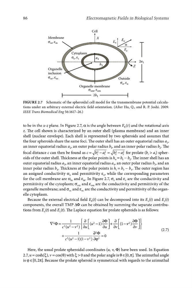
to be in the x-z plane. In Figure 2.7, α is the angle between E 0 (t ) and the rotational axis
z. The cell shown is characterized by an outer shell (plasma membrane) and an inner
shell (nuclear envelope). Each shell is represented by two spheroids and assumes that
the four spheroids share the same foci. The outer shell has an outer equatorial radius a 1 ,
an inner equatorial radius a 2 , an outer polar radius b 1 , and an inner polar radius b 2 . The
focal distance c can then be found as c = b
2
−
2
2
1
a 1 = b 2 − a 2
2
for prolate (b i > a i ) spheroids of the outer shell. Thickness at the polar points is h o = b 1 − b 2 . The inner shell has an
outer equatorial radius a 3 , an inner equatorial radius a 4 , an outer polar radius b 3 , and an
inner polar radius b 4 . Thickness at the polar points is h i = b 3 − b 4 . The outer region has
an assigned conductivity α o and permittivity ε o , while the corresponding parameters
for the cell membrane are α m and ε m . In Figure 2.7, σ c and ε c are the conductivity and
permittivity of the cytoplasm; σ om and ε om are the conductivity and permittivity of the
organelle membrane; and σ oc and ε oc are the conductivity and permittivity of the organelle cytoplasm.
Because the external electrical field E 0 (t) can be decomposed into its E x (t) and E z (t)
components, the overall TMP ∆Φ can be obtained by summing the separate contributions from E x (t) and E z (t). The Laplace equation for prolate spheroids is as follows:
2
1
⎧ ∂ ⎡
Φ
⎤ ∂ ⎡
∂ Φ ⎤⎫
∇ Φ =
⎨
(u
2
∂
−1)
⎢
+
v
c
2
(1 −
2
⎢
v
2
)
⎬
(
⎥
⎥
u − v
2
) ⎩ ∂u ⎣
∂u ⎦
∂v ⎣
∂v ⎦⎭
(2.7)
1
∂ ∂
2
Φ
+
= 0
c
2
(u
2
−1)(1 − v
2
) ∂ϕ
2
Here, the usual prolate spheroidal coordinates (u, v, Φ) have been used. In Equation
2.7, u = cosh( ξ ), v = cos(θ) with ξ > 0 and the polar angle is θ ∈[0 ,π]. The azimuthal angle
is ϕ ∈[0 ,2π]. Because the prolate spheroid is symmetrical with regards to the azimuthal
86
Electromagnetic Fields in Biological Systems
Organelle membrane
Organelle
inclusion
σ oc , ε oc
Outside
σ o , ε o
Cell
Membrane
σ m , ε m
Cytoplasm
σ c , ε c
X
Z
α
2b 1
2a 1
a 3
b 3
σ om , ε om
E z
E x
E o
Figure 2.7 Schematic of the spheroidal cell model for the transmembrane potential calculations under an arbitrary external electric field orientation. (After Hu, Q., and R. P. Joshi. 2009.
IEEE Trans Biomedical Eng 56:1617–26.)
z. The cell shown is characterized by an outer shell (plasma membrane) and an inner
shell (nuclear envelope). Each shell is represented by two spheroids and assumes that
the four spheroids share the same foci. The outer shell has an outer equatorial radius a 1 ,
an inner equatorial radius a 2 , an outer polar radius b 1 , and an inner polar radius b 2 . The
focal distance c can then be found as c = b
2
−
2
2
1
a 1 = b 2 − a 2
2
for prolate (b i > a i ) spheroids of the outer shell. Thickness at the polar points is h o = b 1 − b 2 . The inner shell has an
outer equatorial radius a 3 , an inner equatorial radius a 4 , an outer polar radius b 3 , and an
inner polar radius b 4 . Thickness at the polar points is h i = b 3 − b 4 . The outer region has
an assigned conductivity α o and permittivity ε o , while the corresponding parameters
for the cell membrane are α m and ε m . In Figure 2.7, σ c and ε c are the conductivity and
permittivity of the cytoplasm; σ om and ε om are the conductivity and permittivity of the
organelle membrane; and σ oc and ε oc are the conductivity and permittivity of the organelle cytoplasm.
Because the external electrical field E 0 (t) can be decomposed into its E x (t) and E z (t)
components, the overall TMP ∆Φ can be obtained by summing the separate contributions from E x (t) and E z (t). The Laplace equation for prolate spheroids is as follows:
2
1
⎧ ∂ ⎡
Φ
⎤ ∂ ⎡
∂ Φ ⎤⎫
∇ Φ =
⎨
(u
2
∂
−1)
⎢
+
v
c
2
(1 −
2
⎢
v
2
)
⎬
(
⎥
⎥
u − v
2
) ⎩ ∂u ⎣
∂u ⎦
∂v ⎣
∂v ⎦⎭
(2.7)
1
∂ ∂
2
Φ
+
= 0
c
2
(u
2
−1)(1 − v
2
) ∂ϕ
2
Here, the usual prolate spheroidal coordinates (u, v, Φ) have been used. In Equation
2.7, u = cosh( ξ ), v = cos(θ) with ξ > 0 and the polar angle is θ ∈[0 ,π]. The azimuthal angle
is ϕ ∈[0 ,2π]. Because the prolate spheroid is symmetrical with regards to the azimuthal
86
Electromagnetic Fields in Biological Systems
Organelle membrane
Organelle
inclusion
σ oc , ε oc
Outside
σ o , ε o
Cell
Membrane
σ m , ε m
Cytoplasm
σ c , ε c
X
Z
α
2b 1
2a 1
a 3
b 3
σ om , ε om
E z
E x
E o
Figure 2.7 Schematic of the spheroidal cell model for the transmembrane potential calculations under an arbitrary external electric field orientation. (After Hu, Q., and R. P. Joshi. 2009.
IEEE Trans Biomedical Eng 56:1617–26.)