

444
M. Group Theory
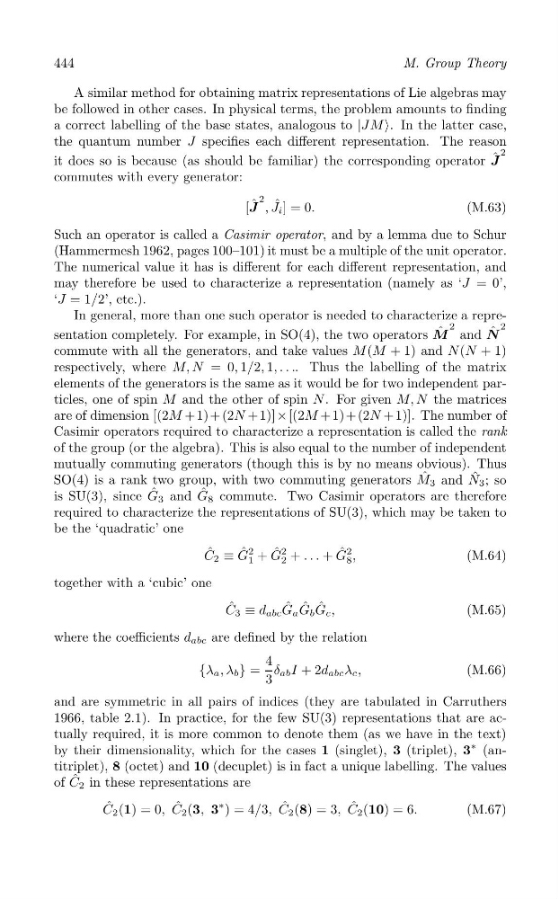
A similar method for obtaining matrix representations of Lie algebras may
be followed in other cases. In physical terms, the problem amounts to finding
a correct labelling of the base states, analogous to |JM ›. In the latter case,
the quantum number J specifies each different representation. The reason
2
it does so is because (as should be familiar) the corresponding operator J ˆ
commutes with every generator:
2
[J ˆ , J ˆ i ] = 0.
(M.63)
Such an operator is called a Casimir operator, and by a lemma due to Schur
(Hammermesh 1962, pages 100–101) it must be a multiple of the unit operator.
The numerical value it has is different for each different representation, and
may therefore be used to characterize a representation (namely as ‘J = 0’,
‘J = 1/2’, etc.).
In general, more than one such operator is needed to characterize a repre2
2
sentation completely. For example, in SO(4), the two operators M ˆ and N ˆ
commute with all the generators, and take values M (M + 1) and N (N + 1)
respectively, where M, N = 0, 1/2, 1, . . .. Thus the labelling of the matrix
elements of the generators is the same as it would be for two independent particles, one of spin M and the other of spin N . For given M, N the matrices
are of dimension [(2M + 1)+ (2N + 1)]× [(2M + 1)+ (2N + 1)]. The number of
Casimir operators required to characterize a representation is called the rank
of the group (or the algebra). This is also equal to the number of independent
mutually commuting generators (though this is by no means obvious). Thus
SO(4) is a rank two group, with two commuting generators M ˆ 3 and N ˆ 3 ; so
is SU(3), since G ˆ 3 and G ˆ 8 commute. Two Casimir operators are therefore
required to characterize the representations of SU(3), which may be taken to
be the ‘quadratic’ one
C ˆ 2 ≡ G ˆ
1
2 + G ˆ
2
2 + . . . + G ˆ
8
2 ,
(M.64)
together with a ‘cubic’ one
ˆ
ˆ ˆ ˆ
C 3 ≡ d abc G a G b G c ,
(M.65)
where the coefficients d abc are defined by the relation
4
{λ a , λ b } = δ ab I + 2d abc λ c ,
(M.66)
3
and are symmetric in all pairs of indices (they are tabulated in Carruthers
1966, table 2.1). In practice, for the few SU(3) representations that are actually required, it is more common to denote them (as we have in the text)
by their dimensionality, which for the cases 1 (singlet), 3 (triplet), 3
∗ (antitriplet), 8 (octet) and 10 (decuplet) is in fact a unique labelling. The values
of C ˆ 2 in these representations are
C ˆ 2 (1) = 0, C ˆ 2 (3, 3
∗ ) = 4/3, C ˆ 2 (8) = 3, C ˆ 2 (10) = 6.
(M.67)
M. Group Theory
A similar method for obtaining matrix representations of Lie algebras may
be followed in other cases. In physical terms, the problem amounts to finding
a correct labelling of the base states, analogous to |JM ›. In the latter case,
the quantum number J specifies each different representation. The reason
2
it does so is because (as should be familiar) the corresponding operator J ˆ
commutes with every generator:
2
[J ˆ , J ˆ i ] = 0.
(M.63)
Such an operator is called a Casimir operator, and by a lemma due to Schur
(Hammermesh 1962, pages 100–101) it must be a multiple of the unit operator.
The numerical value it has is different for each different representation, and
may therefore be used to characterize a representation (namely as ‘J = 0’,
‘J = 1/2’, etc.).
In general, more than one such operator is needed to characterize a repre2
2
sentation completely. For example, in SO(4), the two operators M ˆ and N ˆ
commute with all the generators, and take values M (M + 1) and N (N + 1)
respectively, where M, N = 0, 1/2, 1, . . .. Thus the labelling of the matrix
elements of the generators is the same as it would be for two independent particles, one of spin M and the other of spin N . For given M, N the matrices
are of dimension [(2M + 1)+ (2N + 1)]× [(2M + 1)+ (2N + 1)]. The number of
Casimir operators required to characterize a representation is called the rank
of the group (or the algebra). This is also equal to the number of independent
mutually commuting generators (though this is by no means obvious). Thus
SO(4) is a rank two group, with two commuting generators M ˆ 3 and N ˆ 3 ; so
is SU(3), since G ˆ 3 and G ˆ 8 commute. Two Casimir operators are therefore
required to characterize the representations of SU(3), which may be taken to
be the ‘quadratic’ one
C ˆ 2 ≡ G ˆ
1
2 + G ˆ
2
2 + . . . + G ˆ
8
2 ,
(M.64)
together with a ‘cubic’ one
ˆ
ˆ ˆ ˆ
C 3 ≡ d abc G a G b G c ,
(M.65)
where the coefficients d abc are defined by the relation
4
{λ a , λ b } = δ ab I + 2d abc λ c ,
(M.66)
3
and are symmetric in all pairs of indices (they are tabulated in Carruthers
1966, table 2.1). In practice, for the few SU(3) representations that are actually required, it is more common to denote them (as we have in the text)
by their dimensionality, which for the cases 1 (singlet), 3 (triplet), 3
∗ (antitriplet), 8 (octet) and 10 (decuplet) is in fact a unique labelling. The values
of C ˆ 2 in these representations are
C ˆ 2 (1) = 0, C ˆ 2 (3, 3
∗ ) = 4/3, C ˆ 2 (8) = 3, C ˆ 2 (10) = 6.
(M.67)