

265
19.3. Spontaneously broken local U(1) symmetry
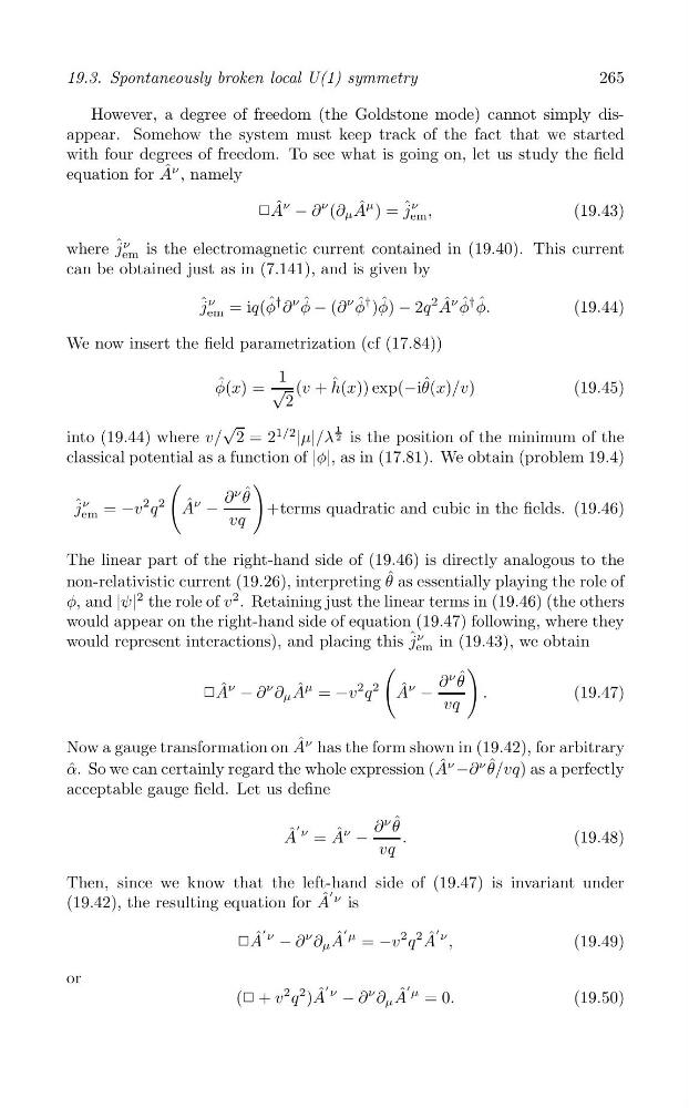
However, a degree of freedom (the Goldstone mode) cannot simply disappear. Somehow the system must keep track of the fact that we started
with four degrees of freedom. To see what is going on, let us study the field
equation for A ˆ ν , namely
❗A ˆ ν − ∂
ν (∂ μ A ˆ μ ) = ˆ j
ν ,
(19.43)
em
where ˆ j
ν is the electromagnetic current contained in (19.40). This current
em
can be obtained just as in (7.141), and is given by
ˆ j
ν
φ
† ∂
ν ˆ
φ
† )φ ˆ ) − 2q
2 A ˆ ν ˆ φ.
(19.44)
= iq( ˆ φ − (∂
ν ˆ
φ
† ˆ
em
We now insert the field parametrization (cf (17.84))
φ ˆ (x) = √
1 (v + h ˆ (x)) exp(−iθ ˆ (x)/v)
(19.45)
2
√
2
into (19.44) where v/ 2 = 2
1/2
|μ|/λ
1 is the position of the minimum of the
classical potential as a function of |φ|, as in (17.81). We obtain (problem 19.4)
(
)
2 2
ˆ j
ν = −v q A ˆ ν −
∂
ν θ ˆ
+terms quadratic and cubic in the fields. (19.46)
em
vq
The linear part of the right-hand side of (19.46) is directly analogous to the
non-relativistic current (19.26), interpreting θ ˆ as essentially playing the role of
φ, and |ψ|
2 the role of v
2 . Retaining just the linear terms in (19.46) (the others
would appear on the right-hand side of equation (19.47) following, where they
would represent interactions), and placing this ˆ j
ν in (19.43), we obtain
em
(
)
2 2
❗A ˆ ν − ∂
ν ∂ μ A ˆ μ = −v q A ˆ ν −
∂
ν θ ˆ
.
(19.47)
vq
Now a gauge transformation on A ˆ ν has the form shown in (19.42), for arbitrary
α ˆ. So we can
A
ν
−∂
ν ˆ
as a perfectly
certainly regard the whole expression ( ˆ
θ/vq)
acceptable gauge field. Let us define
′
∂
ν θ ˆ
ν
A ˆ = A ˆ ν −
.
(19.48)
vq
Then, since we know that the left-hand side of (19.47) is invariant under
ν
(19.42), the resulting equation for A ˆ
′
is
′
′
′
ˆ μ
2 2 ˆ ν
❗A ˆ ν − ∂
ν ∂ μ A = −v q A ,
(19.49)
or
2
(❗ + v q
2 )A ˆ
′ ν
− ∂
ν ∂ μ A ˆ
′ μ = 0.
(19.50)