

188
16. Lattice Field Theory, and the Renormalization Group Revisited
f π
f K
3M Ξ − M N
2M Bs − M Υ
ψ(1P − 1S)
Υ(1D − 1S)
Υ(2P − 1S)
Υ(3S − 1S)
Υ(1P − 1S)
LQCD/Exp’t (n f = 0)
1.1
1
0.9
LQCD/Exp’t (n f = 3)
1.1
1
0.9
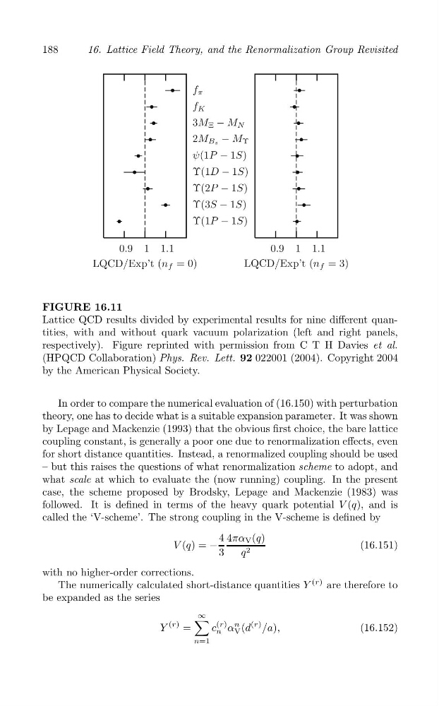
FIGURE 16.11
Lattice QCD results divided by experimental results for nine different quantities, with and without quark vacuum polarization (left and right panels,
respectively). Figure reprinted with permission from C T H Davies et al.
(HPQCD Collaboration) Phys. Rev. Lett. 92 022001 (2004). Copyright 2004
by the American Physical Society.
In order to compare the numerical evaluation of (16.150) with perturbation
theory, one has to decide what is a suitable expansion parameter. It was shown
by Lepage and Mackenzie (1993) that the obvious first choice, the bare lattice
coupling constant, is generally a poor one due to renormalization effects, even
for short distance quantities. Instead, a renormalized coupling should be used
– but this raises the questions of what renormalization scheme to adopt, and
what scale at which to evaluate the (now running) coupling. In the present
case, the scheme proposed by Brodsky, Lepage and Mackenzie (1983) was
followed. It is defined in terms of the heavy quark potential V (q), and is
called the ‘V-scheme’. The strong coupling in the V-scheme is defined by
4 4πα
V (q) = −
V (q)
(16.151)
3
q 2
with no higher-order corrections.
The numerically calculated short-distance quantities Y
(r) are therefore to
be expanded as the series
∑ ∞
Y
(r) =
c
(r) α
n
r
V (d
( )
n
/a),
(16.152)
n=1