

183
16.5. Lattice QCD
g L suitably, so as to ensure that M remains finite. This is, of course, quite
analogous to saying that, in a renormalizable theory, the bare parameters of
the theory depend on the momentum cut-off Λ in such a way that, as Λ → ∞,
finite values are obtained for the corresponding physical parameters (see the
last paragraph of section 10.1.2, for example). In practice, of course, the
extent to which the lattice ‘a’ can really be taken to be very small is severely
limited by the computational resources available – that is, essentially, by the
number of mesh points N .
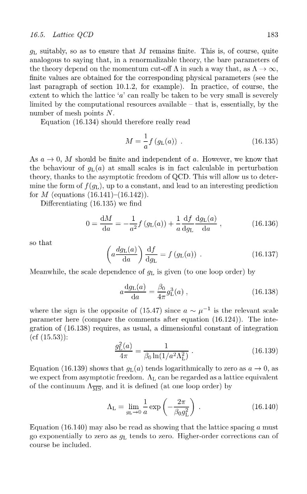
Equation (16.134) should therefore really read
1
M = f (g L (a)) .
(16.135)
a
As a → 0, M should be finite and independent of a. However, we know that
the behaviour of g L (a) at small scales is in fact calculable in perturbation
theory, thanks to the asymptotic freedom of QCD. This will allow us to determine the form of f (g L ), up to a constant, and lead to an interesting prediction
for M (equations (16.141)–(16.142)).
Differentiating (16.135) we find
dM
1
1 df dg L (a)
0 =
= − f (g L (a)) +
,
(16.136)
da
a 2
a dg L da
so that
(
)
dg L (a) df
a
= f (g L (a)) .
(16.137)
da
dg L
Meanwhile, the scale dependence of g L is given (to one loop order) by
dg L (a)
β 0 3
a
=
g L (a) ,
(16.138)
da
4π
where the sign is the opposite of (15.47) since a ∼ μ
−1 is the relevant scale
parameter here (compare the comments after equation (16.124)). The integration of (16.138) requires, as usual, a dimensionful constant of integration
(cf (15.53)):
2
g (a)
1
L
=
.
(16.139)
4π
β 0 ln(1/a 2 Λ 2 )
L
Equation (16.139) shows that g L (a) tends logarithmically to zero as a → 0, as
we expect from asymptotic freedom. Λ L can be regarded as a lattice equivalent
of the continuum Λ , and it is defined (at one loop order) by
MS
(
)
1
2π
Λ L ≡ lim exp −
.
(16.140)
2
gL →0 a
β 0 g L
Equation (16.140) may also be read as showing that the lattice spacing a must
go exponentially to zero as g L tends to zero. Higher-order corrections can of
course be included.