

168
16. Lattice Field Theory, and the Renormalization Group Revisited
where
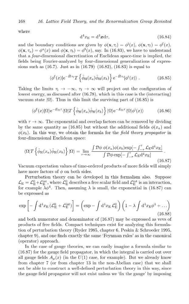
d
4 x E = d
3
xdτ,
(16.84)
and the boundary conditions are given by φ(x, τ i ) = φ
i (x), φ(x, τ f ) = φ
f (x),
φ(x, τ ) = φ
a
b
a
(x) and φ(x, τ b ) = φ (x), say. In (16.83), we have to understand
that a four-dimensional discretization of Euclidean space-time is implied, the
fields being Fourier-analyzed by four-dimensional generalizations of expressions such as (16.7). Just as in (16.79)–(16.82), (16.83) is equal to
{
}
‹φ
f (x)|e
− ˆ
Hτ f
ˆ
ˆ
ˆ
T φ H (x a )φ H (x b ) e
−Hτi
|φ
i (x)› .
(16.85)
Taking the limits τ i → −∞, τ f → ∞ will project out the configuration of
lowest energy, as discussed after (16.78), which in this case is the (interacting)
vacuum state |Ω›. Thus in this limit the surviving part of (16.85) is
{
}
‹φ
f (x)|Ω›e
−EΩτ
‹ |
ˆ
ˆ
Ω T φ H (x a )φ H (x b ) |Ω›e
−EΩτ
‹Ω|φ
i (x)›
(16.86)
with τ → ∞. The exponential and overlap factors can be removed by dividing
by the same quantity as (16.85) but without the additional fields φ(x a ) and
φ(x b ). In this way, we obtain the formula for the field theory propagator in
four-dimensional Euclidean space:
∫
∫
{
}
Dφ φ(x a )φ(x b )exp[
ˆ
ˆ
Ω T φ H (x a )φ H (x b ) Ω = lim
∫
∫ τ
−
τ
|
| ›
−τ L E d
4 x E ]
‹
.
τ →∞
Dφ exp[− −τ L E d 4 x E ]
(16.87)
Vacuum expectation values of time-ordered products of more fields will simply
have more factors of φ on both sides.
Perturbation theory can be developed in this formalism also. Suppose
L E = L
0
E +L
int
E , where L
0
E describes a free scalar field and L
int
E is an interaction,
for example λφ
4 . Then, assuming λ is small, the exponential in (16.87) can
be expressed as
[ ∫
] (
∫
) (
∫
)
exp − d
4 x (L
0
E + L
int
E
E ) = exp − d
4 x
0
4
E L E
1 − λ d x E φ
4 + . . .
(16.88)
and both numerator and denominator of (16.87) may be expressed as vevs of
products of free fields. Compact techniques exist for analyzing this formulation of perturbation theory (Ryder 1985, chapter 6, Peskin & Schroeder 1995,
chapter 9), and one finds exactly the same ‘Feynman rules’ as in the canonical
(operator) approach.
In the case of gauge theories, we can easily imagine a formula similar to
(16.87) for the gauge field propagator, in which the integral is carried out over
all gauge fields A μ (x) (in the U (1) case, for example). But we already know
from chapter 7 (or from chapter 13 in the non-Abelian case) that we shall
not be able to construct a well-defined perturbation theory in this way, since
the gauge field propagator will not exist unless we ‘fix the gauge’ by imposing