163
i
16.3. Representation of quantum amplitudes
which is, indeed, the amplitude for the system described by H ˆ to go from q
f
at t i to q at t f . Using (16.52) we can write
H ‹q
f
|q
i
› H = ‹q
f
|e
−iH ˆ (t f −ti)
|q
i
› ;
(16.55)
t f ti
we want to understand how (16.55) can be represented as (16.49).
We shall demonstrate the connection explicitly for the special case of a
free particle, for which
2
p ˆ
ˆ
H =
.
(16.56)
2m
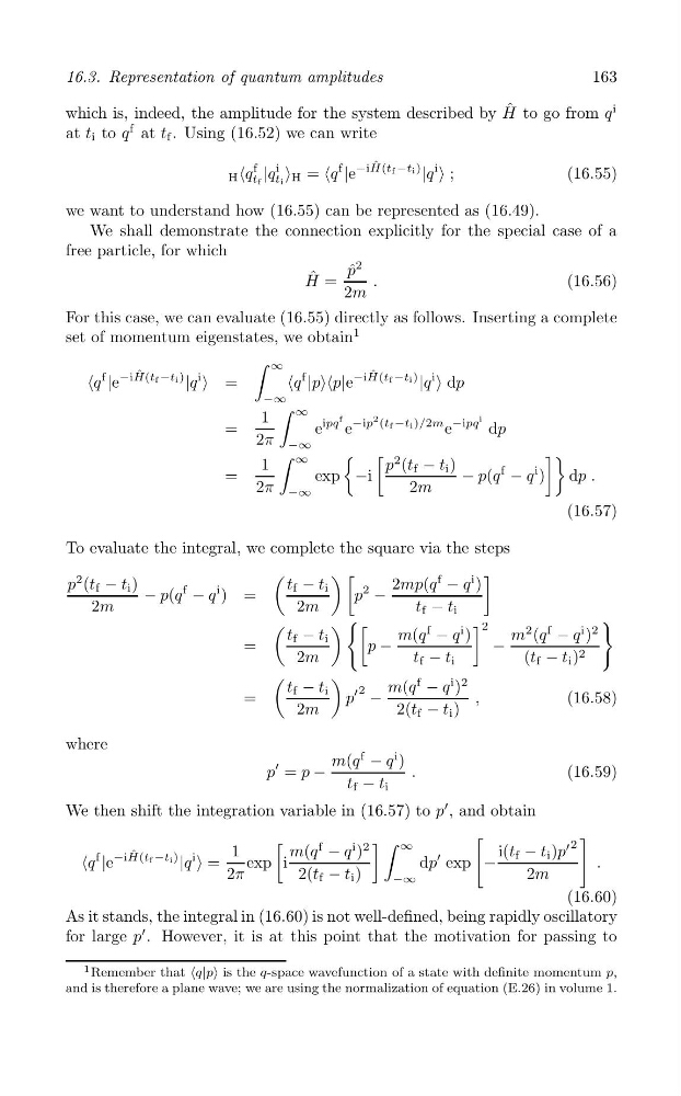
For this case, we can evaluate (16.55) directly as follows. Inserting a complete
set of momentum eigenstates, we obtain
1
∫ ∞
‹q
f
|e
−iH ˆ (t f −ti)
|q
i
› =
‹q
f
|p›‹p|e
−iH ˆ (t f −ti)
|q
i
› dp
−∞
∫ ∞
f
2
i
1
ipq −ip (t f −ti)/2m −ipq
=
e e
e
dp
2π −∞
∫
( [
])
∞
1
p
2 (t f − t i )
=
exp −i
− p(q
f
− q
i ) dp .
2π
2m
−∞
(16.57)
To evaluate the integral, we complete the square via the steps
(
) [
]
p
2 (t f − t i )
t f − t i
2mp(q
f
− q
i )
− p(q
f
− q
i ) =
p
2
−
2m
2m
t f − t i
(
) ( [
] 2
(
t f − t i
m(q
f
− q
i )
m
2 (q
f
− q
i )
2
=
p −
−
2m
t f − t i
(t f − t i ) 2
(
)
t f − t i
′ 2
m(q
f
− q
i )
2
=
p −
,
(16.58)
2m
2(t f − t i )
where
m(q
f
− q
i )
′
p = p −
.
(16.59)
t f − t i
We then shift the integration variable in (16.57) to p
′ , and obtain
[
] ∫
[
]
∞
′ 2
‹q
f
|e
−iH ˆ (t f −ti)
|q
i
› =
1 exp i
m(q
f
− q
i )
2
dp
′ exp −
i(t f − t i )p
.
2π
2(t f − t i )
2m
−∞
(16.60)
As it stands, the integral in (16.60) is not well-defined, being rapidly oscillatory
′
for large p . However, it is at this point that the motivation for passing to
1 Remember that is the q-space wavefunction of a state with definite momentum p,
and is therefore a plane wave; we are using the normalization of equation (E.26) in volume 1.