

136
15. QCD II: Asymptotic Freedom, the Renormalization Group
corrections to the simple parton model, calculated using RGE techniques, predict observable violations of scaling in deep inelastic scattering. As we shall
see, comparison between the theoretical predictions and experimental measurements provides strong evidence for the correctness of QCD as the theory
of nucleonic constituents.
15.6.1 Uncancelled mass singularities at order α s .
The free parton model amplitudes we considered in chapter 9 for deep inelastic
lepton-nucleon scattering were of the form shown in figure 15.7 (cf figure 9.4).
The obvious first QCD corrections will be due to real gluon emission by either
the initial or final quark, as shown in figure 15.8, but to these we must add the
one-loop virtual gluon processes of figure 15.9 in order (see below) to get rid
of infrared divergences similar to those encountered in section 14.4.2, and also
the diagram of figure 15.10, corresponding to the presence of gluons in the
nucleon. To simplify matters, we shall consider what is called a ‘non-singlet
F
ep −F
en
structure function’ F 2
NS , such as
2 in which the (flavour) singlet gluon
2
contribution cancels out, leaving only the diagrams of figures 15.8 and 15.9.
We now want to perform, for these diagrams, calculations analogous to
those of section 9.2, which enabled us to find the e-N structure functions
νW 2 and M W 1 from the simple parton process of figure 15.7. There are two
problems here: one is to find the parton level W ’s corresponding to figure
15.8 (leaving aside figure 15.9 for the moment) – cf equations (9.29) and
(9.30) in the case of the free parton diagram figure 15.7; the other is to relate
these parton W ’s to observed nucleon W ’s via an integration over momentum
fractions. In section 9.2 we solved the first problem by explicitly calculating
the parton level d
2 σ
i /dQ
2 dν and picking off the associated νW 2
i , W 1
i . In
principle, the same can be done here, starting from the five-fold differential
cross section for our e
− + q → e
− + q + g process. However, a simpler – if
somewhat heuristic – way is available. We note from (9.46) that in general
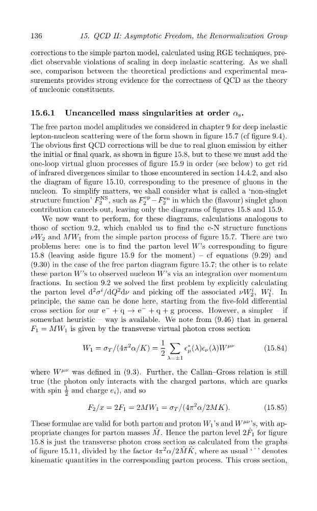
F 1 = M W 1 is given by the transverse virtual photon cross section
∑
1
∈
∗
μ (λ)∈ ν (λ)W
μν
W 1 = σ T /(4π
2 α/K) =
(15.84)
2
λ=±1
where W
μν was defined in (9.3). Further, the Callan–Gross relation is still
true (the photon only interacts with the charged partons, which are quarks
with spin
1 and charge e i ), and so
2
F 2 /x = 2F 1 = 2M W 1 = σ T /(4π
2 α/2M K).
(15.85)
These formulae are valid for both parton and proton W 1 ’s and W
μν ’s, with appropriate changes for parton masses M ˆ . Hence the parton level 2F ˆ 1 for figure
15.8 is just the transverse photon cross section as calculated from the graphs
of figure 15.11, divided by the factor 4π
2 α/2M ˆ K ˆ , where as usual ‘ˆ’ denotes
kinematic quantities in the corresponding parton process. This cross section,