

133
15.5. A more general form of the RGE
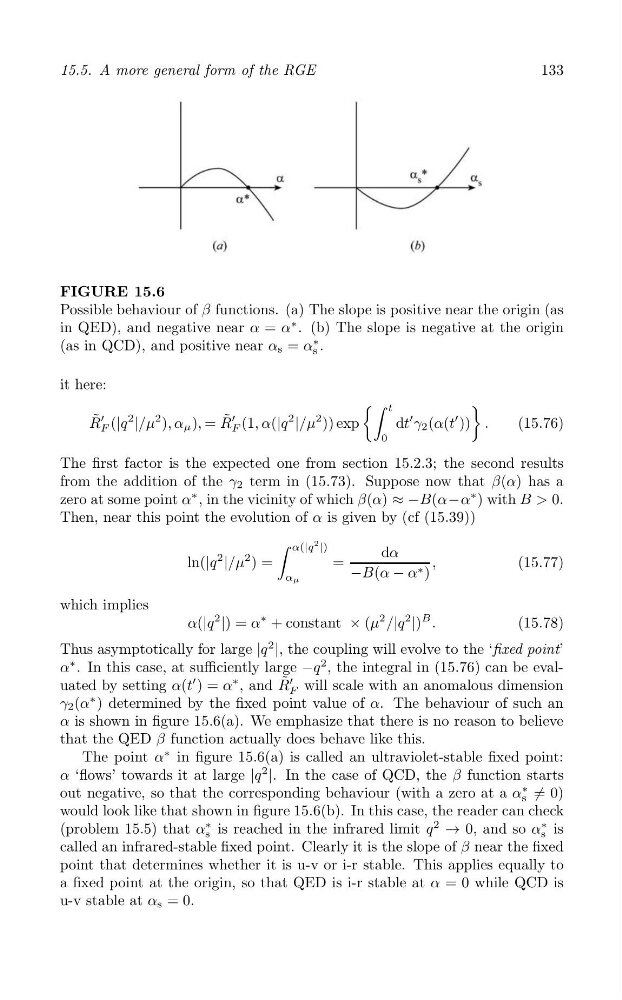
FIGURE 15.6
Possible behaviour of β functions. (a) The slope is positive near the origin (as
in QED), and negative near α = α
∗ . (b) The slope is negative at the origin
(as in QCD), and positive near α s = α
∗ .
s
it here:
(∫
)
t
R ˜ ′
R ˜ ′
F (|q
2
|/μ
2 ), α μ ), = F (1, α(|q
2
|/μ
2 )) exp
dt
′ γ 2 (α(t
′ )) .
(15.76)
0
The first factor is the expected one from section 15.2.3; the second results
from the addition of the γ 2 term in (15.73). Suppose now that β(α) has a
zero at some point α
∗ , in the vicinity of which β(α) ≈ −B(α−α
∗ ) with B > 0.
Then, near this point the evolution of α is given by (cf (15.39))
∫ α(|q
2 |)
dα
ln(|q
2
|/μ
2 ) =
=
,
(15.77)
αμ
−B(α − α ∗ )
which implies
α(|q
2
|) = α
∗ + constant × (μ
2 /|q
2
|)
B .
(15.78)
Thus asymptotically for large |q
2
|, the coupling will evolve to the ‘fixed point’
α
∗ . In this case, at sufficiently large −q
2 , the integral in (15.76) can be evaluated by setting α(t
′ ) = α
∗ , and R ˜ ′ will scale with an anomalous dimension
F
γ 2 (α
∗ ) determined by the fixed point value of α. The behaviour of such an
α is shown in figure 15.6(a). We emphasize that there is no reason to believe
that the QED β function actually does behave like this.
The point α
∗ in figure 15.6(a) is called an ultraviolet-stable fixed point:
α ‘flows’ towards it at large |q
2
|. In the case of QCD, the β function starts
out negative, so that the corresponding behaviour (with a zero at a α
∗
/ = 0)
s
would look like that shown in figure 15.6(b). In this case, the reader can check
2
(problem 15.5) that α
∗ is reached in the infrared limit q → 0, and so α
∗ is
s
s
called an infrared-stable fixed point. Clearly it is the slope of β near the fixed
point that determines whether it is u-v or i-r stable. This applies equally to
a fixed point at the origin, so that QED is i-r stable at α = 0 while QCD is
u-v stable at α s = 0.