

406
I. The Schr¨ odinger and Heisenberg Pictures
the operator U ˆ = exp(−i ˆ
Ht) is unitary:
U
† = [exp(−iHt ˆ )]
† = exp(i H ˆ †
Ht) = U
−1
t) = exp(i ˆ
(I.5)
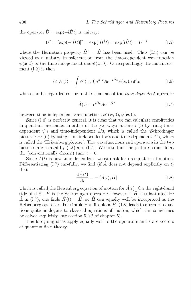
where the Hermitian property H ˆ † = H ˆ has been used. Thus (I.3) can be
viewed as a unitary transformation from the time-dependent wavefunction
ψ(x, t) to the time-independent one ψ(x, 0). Correspondingly the matrix element (I.2) is then
∫
Ht ˆ −i ˆ
<φ|A ˆ |ψ> = φ
∗ (x, 0)e
i ˆ Ae
Ht ψ(x, 0) d
3
x
(I.6)
which can be regarded as the matrix element of the time-dependent operator
ˆ
iHt ˆ ˆ −i ˆ
Ht
A(t) = e Ae
(I.7)
between time-independent wavefunctions φ
∗ (x, 0), ψ(x, 0).
Since (I.6) is perfectly general, it is clear that we can calculate amplitudes
in quantum mechanics in either of the two ways outlined: (i) by using timedependent ψ’s and time-independent A ˆ ’s, which is called the ‘Schr¨ odinger
picture’: or (ii) by using time-independent ψ’s and time-dependent A ˆ ’s, which
is called the ‘Heisenberg picture’. The wavefunctions and operators in the two
pictures are related by (I.3) and (I.7). We note that the pictures coincide at
the (conventionally chosen) time t = 0.
Since A ˆ (t) is now time-dependent, we can ask for its equation of motion.
Differentiating (I.7) carefully, we find (if A ˆ does not depend explicitly on t)
that
dA ˆ (t) = −i[A ˆ (t), H ˆ ]
( I . 8 )
dt
which is called the Heisenberg equation of motion for A ˆ (t). On the right-hand
side of (I.8), H ˆ is the Schr¨ odinger operator; however, if H ˆ is substituted for
A ˆ in (I.7), one finds H ˆ (t) = H ˆ , so H ˆ can equally well be interpreted as the
Heisenberg operator. For simple Hamiltonians H ˆ , (I.8) leads to operator equations quite analogous to classical equations of motion, which can sometimes
be solved explicitly (see section 5.2.2 of chapter 5).
The foregoing ideas apply equally well to the operators and state vectors
of quantum field theory.
I. The Schr¨ odinger and Heisenberg Pictures
the operator U ˆ = exp(−i ˆ
Ht) is unitary:
U
† = [exp(−iHt ˆ )]
† = exp(i H ˆ †
Ht) = U
−1
t) = exp(i ˆ
(I.5)
where the Hermitian property H ˆ † = H ˆ has been used. Thus (I.3) can be
viewed as a unitary transformation from the time-dependent wavefunction
ψ(x, t) to the time-independent one ψ(x, 0). Correspondingly the matrix element (I.2) is then
∫
Ht ˆ −i ˆ
<φ|A ˆ |ψ> = φ
∗ (x, 0)e
i ˆ Ae
Ht ψ(x, 0) d
3
x
(I.6)
which can be regarded as the matrix element of the time-dependent operator
ˆ
iHt ˆ ˆ −i ˆ
Ht
A(t) = e Ae
(I.7)
between time-independent wavefunctions φ
∗ (x, 0), ψ(x, 0).
Since (I.6) is perfectly general, it is clear that we can calculate amplitudes
in quantum mechanics in either of the two ways outlined: (i) by using timedependent ψ’s and time-independent A ˆ ’s, which is called the ‘Schr¨ odinger
picture’: or (ii) by using time-independent ψ’s and time-dependent A ˆ ’s, which
is called the ‘Heisenberg picture’. The wavefunctions and operators in the two
pictures are related by (I.3) and (I.7). We note that the pictures coincide at
the (conventionally chosen) time t = 0.
Since A ˆ (t) is now time-dependent, we can ask for its equation of motion.
Differentiating (I.7) carefully, we find (if A ˆ does not depend explicitly on t)
that
dA ˆ (t) = −i[A ˆ (t), H ˆ ]
( I . 8 )
dt
which is called the Heisenberg equation of motion for A ˆ (t). On the right-hand
side of (I.8), H ˆ is the Schr¨ odinger operator; however, if H ˆ is substituted for
A ˆ in (I.7), one finds H ˆ (t) = H ˆ , so H ˆ can equally well be interpreted as the
Heisenberg operator. For simple Hamiltonians H ˆ , (I.8) leads to operator equations quite analogous to classical equations of motion, which can sometimes
be solved explicitly (see section 5.2.2 of chapter 5).
The foregoing ideas apply equally well to the operators and state vectors
of quantum field theory.