

11.8. Which theories are renormalizable – and does it matter?
357
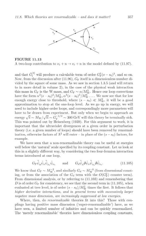
FIGURE 11.13
A two-loop contribution to ν e + n → ν e + n in the model defined by (11.97).
and that G ¯ [3] will produce a calculable term of order G
3 (s − s 0 )
3 , and so on.
l
F
Now, from the discussion after (11.96), G F itself is a dimensionless number divided by the square of some mass. As we saw in section 1.3.5 (and will return
to in more detail in volume 2), in the case of the physical weak interaction
this mass in G F is the W-mass, and G F ∼ α/M
2 . Hence our loop corrections
W
have the form α
2 (s − s 0 )
2 /M
4 , α
3 (s − s 0 )
3 /M
6
. We now see that for low
W . . .
W
enough energy close to threshold, where (s − s 0 ) ≪ M
2 , it will be a good
W
approximation to stop at the one-loop level. As we go up in energy, we will
need to include higher-order loops, and correspondingly more parameters will
have to be drawn from experiment. But only when we begin to approach an
√
√
−1/2
energy s ∼ M W / α ∼ G
∼ 300 GeV will this theory be terminally sick.
F
This was pointed out by Heisenberg (1939). For this argument to work, it is
important that the ultraviolet divergences at a given order in perturbation
theory (i.e. a given number of loops) should have been removed by renormalization, otherwise factors of Λ
2 will enter – in place of the (s − s 0 ) factors, for
example.
We have seen that a non-renormalizable theory can be useful at energies
well below the ‘natural’ scale specified by its coupling constant. Let us look at
this in a slightly different way, by considering the two four-fermion interaction
terms introduced at one loop,
¯
¯
¯
¯
ˆ ˆ ˆ ˆ
ˆ ∂ / ˆ ˆ ∂ / ˆ
G F ψ ψ n
ψ νe
and
G d ψ ψ n
ψ νe .
(11.105)
n
ψ νe
n
ψ νe
We know that G F ∼ M
−2 and similarly G d ∼ M
−4 (from dimensional countW ,
W
ing, or from the association of the G d term with the O(G
2 ) counter term).
F
From dimensional analysis, or by referring to (11.103) and remembering that
D is of order G F for consistency, we see that the second term in (11.105), when
evaluated at tree level, is of order (s − s 0 )/M
2 times the first. It follows that
W
higher derivative interactions, and in general terms with successively larger
negative mass dimension, are increasingly suppressed at low energies.
Where, then, do renormalizable theories fit into this? Those with couplings having positive mass dimension (‘super-renormalizable’) have, as we
have seen, a limited number of infinities and can be quickly renormalized.
The ‘merely renormalizable’ theories have dimensionless coupling constants,
357
FIGURE 11.13
A two-loop contribution to ν e + n → ν e + n in the model defined by (11.97).
and that G ¯ [3] will produce a calculable term of order G
3 (s − s 0 )
3 , and so on.
l
F
Now, from the discussion after (11.96), G F itself is a dimensionless number divided by the square of some mass. As we saw in section 1.3.5 (and will return
to in more detail in volume 2), in the case of the physical weak interaction
this mass in G F is the W-mass, and G F ∼ α/M
2 . Hence our loop corrections
W
have the form α
2 (s − s 0 )
2 /M
4 , α
3 (s − s 0 )
3 /M
6
. We now see that for low
W . . .
W
enough energy close to threshold, where (s − s 0 ) ≪ M
2 , it will be a good
W
approximation to stop at the one-loop level. As we go up in energy, we will
need to include higher-order loops, and correspondingly more parameters will
have to be drawn from experiment. But only when we begin to approach an
√
√
−1/2
energy s ∼ M W / α ∼ G
∼ 300 GeV will this theory be terminally sick.
F
This was pointed out by Heisenberg (1939). For this argument to work, it is
important that the ultraviolet divergences at a given order in perturbation
theory (i.e. a given number of loops) should have been removed by renormalization, otherwise factors of Λ
2 will enter – in place of the (s − s 0 ) factors, for
example.
We have seen that a non-renormalizable theory can be useful at energies
well below the ‘natural’ scale specified by its coupling constant. Let us look at
this in a slightly different way, by considering the two four-fermion interaction
terms introduced at one loop,
¯
¯
¯
¯
ˆ ˆ ˆ ˆ
ˆ ∂ / ˆ ˆ ∂ / ˆ
G F ψ ψ n
ψ νe
and
G d ψ ψ n
ψ νe .
(11.105)
n
ψ νe
n
ψ νe
We know that G F ∼ M
−2 and similarly G d ∼ M
−4 (from dimensional countW ,
W
ing, or from the association of the G d term with the O(G
2 ) counter term).
F
From dimensional analysis, or by referring to (11.103) and remembering that
D is of order G F for consistency, we see that the second term in (11.105), when
evaluated at tree level, is of order (s − s 0 )/M
2 times the first. It follows that
W
higher derivative interactions, and in general terms with successively larger
negative mass dimension, are increasingly suppressed at low energies.
Where, then, do renormalizable theories fit into this? Those with couplings having positive mass dimension (‘super-renormalizable’) have, as we
have seen, a limited number of infinities and can be quickly renormalized.
The ‘merely renormalizable’ theories have dimensionless coupling constants,