

334
11. Loops and Renormalization II: QED
where
ρ
ρ
P
ρ = g ν −
q q ν
ν
q 2
and
ρ
δ
ρ
g =
ν
ν
(i.e. the 4×4 unit matrix). It is easy to check (problem 10.5) that P τ
ρ P
τ = P
ρ
ν
ν .
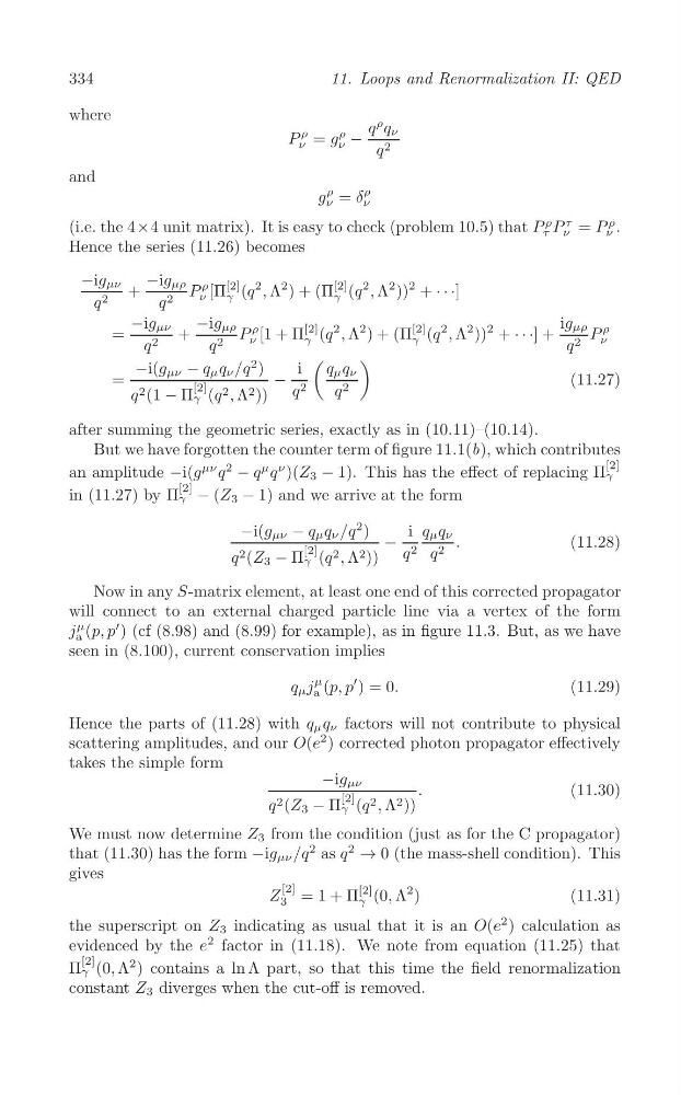
Hence the series (11.26) becomes
−ig μν
−ig μρ P ν
ρ [Π
[2] 2
2
+
(q , Λ
2 ) + (Π
[2] (q , Λ
2 ))
2 + · · ·]
γ
γ
q 2
q 2
−ig μν
−ig μρ
2
2
ig μρ
=
+
P ν
ρ [1 + Π
[2] (q , Λ
2 ) + (Π
[2] (q , Λ
2 ))
2 + · · ·] +
P
ρ
γ
γ
ν
q 2
q 2
q 2
(
)
−i(g μν − q μ q ν /q
2 )
i q μ q ν
=
−
(11.27)
[2]
q 2
q 2
q 2 (1 − Π γ (q 2 , Λ 2 ))
after summing the geometric series, exactly as in (10.11)–(10.14).
But we have forgotten the counter term of figure 11.1(b), which contributes
[2]
μν
μ
an amplitude −i(g q
2
− q q
ν )(Z 3 − 1). This has the effect of replacing Π γ
[2]
in (11.27) by Π γ − (Z 3 − 1) and we arrive at the form
−i(g μν − q μ q ν /q
2 )
i q μ q ν
−
.
(11.28)
[2]
q 2 q 2
q 2 (Z 3 − Π γ (q 2 , Λ 2 ))
Now in any S-matrix element, at least one end of this corrected propagator
will connect to an external charged particle line via a vertex of the form
j
μ (p, p
′ ) (cf (8.98) and (8.99) for example), as in figure 11.3. But, as we have
a
seen in (8.100), current conservation implies
q μ j
μ (p, p
′ ) = 0.
(11.29)
a
Hence the parts of (11.28) with q μ q ν factors will not contribute to physical
scattering amplitudes, and our O(e
2 ) corrected photon propagator effectively
takes the simple form
−ig μν
.
(11.30)
[2]
q 2 (Z 3 − Π γ (q 2 , Λ 2 ))
We must now determine Z 3 from the condition (just as for the C propagator)
that (11.30) has the form −ig μν /q
2 as q
2
→ 0 (the mass-shell condition). This
gives
Z
[2] = 1 + Π
[2] (0, Λ
2 )
(11.31)
3
γ
the superscript on Z 3 indicating as usual that it is an O(e
2 ) calculation as
2
evidenced by the e factor in (11.18). We note from equation (11.25) that
[2]
Π γ (0, Λ
2 ) contains a ln Λ part, so that this time the field renormalization
constant Z 3 diverges when the cut-off is removed.
11. Loops and Renormalization II: QED
where
ρ
ρ
P
ρ = g ν −
q q ν
ν
q 2
and
ρ
δ
ρ
g =
ν
ν
(i.e. the 4×4 unit matrix). It is easy to check (problem 10.5) that P τ
ρ P
τ = P
ρ
ν
ν .
Hence the series (11.26) becomes
−ig μν
−ig μρ P ν
ρ [Π
[2] 2
2
+
(q , Λ
2 ) + (Π
[2] (q , Λ
2 ))
2 + · · ·]
γ
γ
q 2
q 2
−ig μν
−ig μρ
2
2
ig μρ
=
+
P ν
ρ [1 + Π
[2] (q , Λ
2 ) + (Π
[2] (q , Λ
2 ))
2 + · · ·] +
P
ρ
γ
γ
ν
q 2
q 2
q 2
(
)
−i(g μν − q μ q ν /q
2 )
i q μ q ν
=
−
(11.27)
[2]
q 2
q 2
q 2 (1 − Π γ (q 2 , Λ 2 ))
after summing the geometric series, exactly as in (10.11)–(10.14).
But we have forgotten the counter term of figure 11.1(b), which contributes
[2]
μν
μ
an amplitude −i(g q
2
− q q
ν )(Z 3 − 1). This has the effect of replacing Π γ
[2]
in (11.27) by Π γ − (Z 3 − 1) and we arrive at the form
−i(g μν − q μ q ν /q
2 )
i q μ q ν
−
.
(11.28)
[2]
q 2 q 2
q 2 (Z 3 − Π γ (q 2 , Λ 2 ))
Now in any S-matrix element, at least one end of this corrected propagator
will connect to an external charged particle line via a vertex of the form
j
μ (p, p
′ ) (cf (8.98) and (8.99) for example), as in figure 11.3. But, as we have
a
seen in (8.100), current conservation implies
q μ j
μ (p, p
′ ) = 0.
(11.29)
a
Hence the parts of (11.28) with q μ q ν factors will not contribute to physical
scattering amplitudes, and our O(e
2 ) corrected photon propagator effectively
takes the simple form
−ig μν
.
(11.30)
[2]
q 2 (Z 3 − Π γ (q 2 , Λ 2 ))
We must now determine Z 3 from the condition (just as for the C propagator)
that (11.30) has the form −ig μν /q
2 as q
2
→ 0 (the mass-shell condition). This
gives
Z
[2] = 1 + Π
[2] (0, Λ
2 )
(11.31)
3
γ
the superscript on Z 3 indicating as usual that it is an O(e
2 ) calculation as
2
evidenced by the e factor in (11.18). We note from equation (11.25) that
[2]
Π γ (0, Λ
2 ) contains a ln Λ part, so that this time the field renormalization
constant Z 3 diverges when the cut-off is removed.