

302
10. Loops and Renormalization I: The ABC Theory
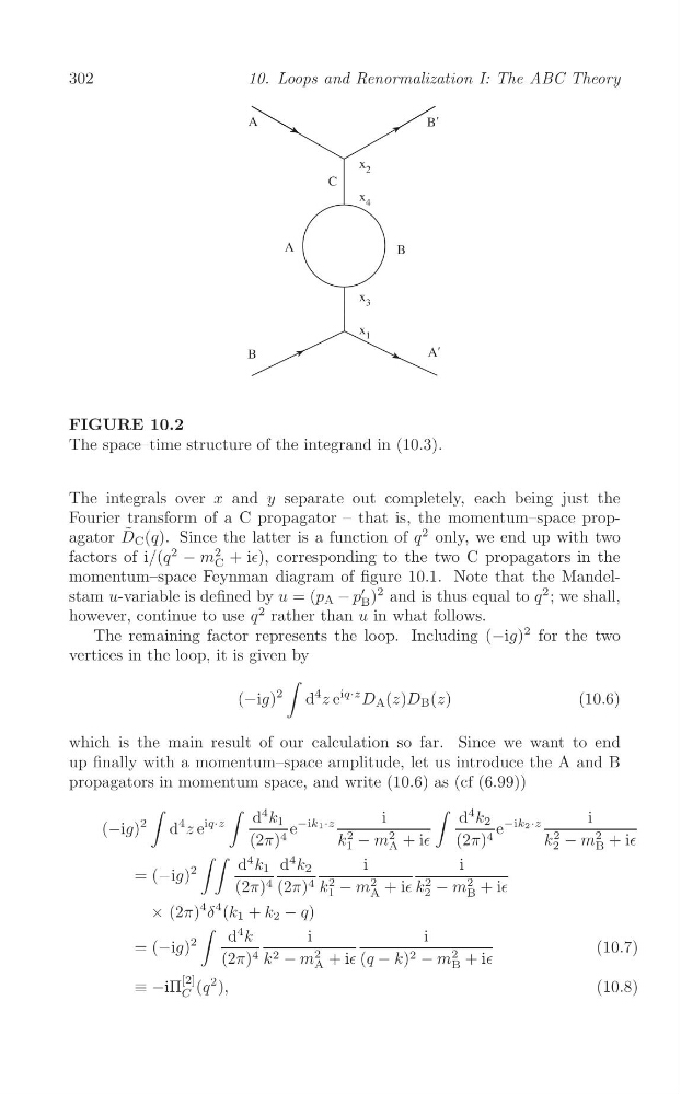
FIGURE 10.2
The space–time structure of the integrand in (10.3).
The integrals over x and y separate out completely, each being just the
Fourier transform of a C propagator – that is, the momentum–space prop2
agator D ˜ C (q). Since the latter is a function of q only, we end up with two
2
− m
2
factors of i/(q
+ i∈), corresponding to the two C propagators in the
C
momentum–space Feynman diagram of figure 10.1. Note that the Mandel′
2
stam u-variable is defined by u = (p A − p )
2 and is thus equal to q ; we shall,
B
however, continue to use q
2 rather than u in what follows.
The remaining factor represents the loop. Including (−ig)
2 for the two
vertices in the loop, it is given by
∫
(−ig)
2
d
4 z e
iq·z D A (z)D B (z)
(10.6)
which is the main result of our calculation so far. Since we want to end
up finally with a momentum–space amplitude, let us introduce the A and B
propagators in momentum space, and write (10.6) as (cf (6.99))
∫
∫
∫
d
4 k 1
i
d
4 k 2
i
iq·z
−ik1 ·z
−ik2 ·z
(−ig)
2
d
4 z e
e
e
k 2
2
k 2
2
(2π) 4
− m + i∈
(2π) 4
− m + i∈
1
A
2
B
∫ ∫ d
4 k 1 d
4 k 2
i
i
= (−ig)
2
k 2
2
k 2
2
(2π) 4 (2π) 4
− m + i∈ − m + i∈
1
A
2
B
× (2π)
4 δ
4 (k 1 + k 2 − q)
∫ d
4 k
i
i
= (−ig)
2
(10.7)
2
2
(2π) 4 k 2 − m + i∈ (q − k) 2 − m + i∈
A
B
≡ −iΠ
[2] (q
2 ),
(10.8)
C
10. Loops and Renormalization I: The ABC Theory
FIGURE 10.2
The space–time structure of the integrand in (10.3).
The integrals over x and y separate out completely, each being just the
Fourier transform of a C propagator – that is, the momentum–space prop2
agator D ˜ C (q). Since the latter is a function of q only, we end up with two
2
− m
2
factors of i/(q
+ i∈), corresponding to the two C propagators in the
C
momentum–space Feynman diagram of figure 10.1. Note that the Mandel′
2
stam u-variable is defined by u = (p A − p )
2 and is thus equal to q ; we shall,
B
however, continue to use q
2 rather than u in what follows.
The remaining factor represents the loop. Including (−ig)
2 for the two
vertices in the loop, it is given by
∫
(−ig)
2
d
4 z e
iq·z D A (z)D B (z)
(10.6)
which is the main result of our calculation so far. Since we want to end
up finally with a momentum–space amplitude, let us introduce the A and B
propagators in momentum space, and write (10.6) as (cf (6.99))
∫
∫
∫
d
4 k 1
i
d
4 k 2
i
iq·z
−ik1 ·z
−ik2 ·z
(−ig)
2
d
4 z e
e
e
k 2
2
k 2
2
(2π) 4
− m + i∈
(2π) 4
− m + i∈
1
A
2
B
∫ ∫ d
4 k 1 d
4 k 2
i
i
= (−ig)
2
k 2
2
k 2
2
(2π) 4 (2π) 4
− m + i∈ − m + i∈
1
A
2
B
× (2π)
4 δ
4 (k 1 + k 2 − q)
∫ d
4 k
i
i
= (−ig)
2
(10.7)
2
2
(2π) 4 k 2 − m + i∈ (q − k) 2 − m + i∈
A
B
≡ −iΠ
[2] (q
2 ),
(10.8)
C