

+ −
9.5. e e annihilation into hadrons
291
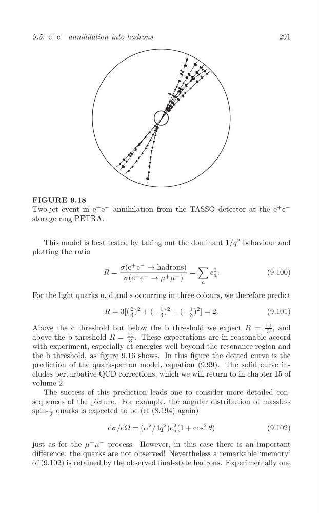
FIGURE 9.18
−
−
Two-jet event in e
+ e annihilation from the TASSO detector at the e
+ e
storage ring PETRA.
This model is best tested by taking out the dominant 1/q
2 behaviour and
plotting the ratio
∑
σ(e
+ e
−
→ hadrons)
2
R =
=
e .
(9.100)
a
σ(e + e − → μ + μ − )
a
For the light quarks u, d and s occurring in three colours, we therefore predict
R = 3[(
2 )
2 + (−
1 )
2 + (−
1 )
2 ] = 2.
(9.101)
3
3
3
10
Above the c threshold but below the b threshold we expect R =
, and
3
11
above the b threshold R = . These expectations are in reasonable accord
3
with experiment, especially at energies well beyond the resonance region and
the b threshold, as figure 9.16 shows. In this figure the dotted curve is the
prediction of the quark-parton model, equation (9.99). The solid curve includes perturbative QCD corrections, which we will return to in chapter 15 of
volume 2.
The success of this prediction leads one to consider more detailed consequences of the picture. For example, the angular distribution of massless
spin1 quarks is expected to be (cf (8.194) again)
2
2
dσ/dΩ = (α
2 /4q
2 )e (1 + cos
2 θ)
(9.102)
a
just as for the μ
+ μ
− process. However, in this case there is an important
difference: the quarks are not observed! Nevertheless a remarkable ‘memory’
of (9.102) is retained by the observed final-state hadrons. Experimentally one
9.5. e e annihilation into hadrons
291
FIGURE 9.18
−
−
Two-jet event in e
+ e annihilation from the TASSO detector at the e
+ e
storage ring PETRA.
This model is best tested by taking out the dominant 1/q
2 behaviour and
plotting the ratio
∑
σ(e
+ e
−
→ hadrons)
2
R =
=
e .
(9.100)
a
σ(e + e − → μ + μ − )
a
For the light quarks u, d and s occurring in three colours, we therefore predict
R = 3[(
2 )
2 + (−
1 )
2 + (−
1 )
2 ] = 2.
(9.101)
3
3
3
10
Above the c threshold but below the b threshold we expect R =
, and
3
11
above the b threshold R = . These expectations are in reasonable accord
3
with experiment, especially at energies well beyond the resonance region and
the b threshold, as figure 9.16 shows. In this figure the dotted curve is the
prediction of the quark-parton model, equation (9.99). The solid curve includes perturbative QCD corrections, which we will return to in chapter 15 of
volume 2.
The success of this prediction leads one to consider more detailed consequences of the picture. For example, the angular distribution of massless
spin1 quarks is expected to be (cf (8.194) again)
2
2
dσ/dΩ = (α
2 /4q
2 )e (1 + cos
2 θ)
(9.102)
a
just as for the μ
+ μ
− process. However, in this case there is an important
difference: the quarks are not observed! Nevertheless a remarkable ‘memory’
of (9.102) is retained by the observed final-state hadrons. Experimentally one