

266
8. Elementary Processes in Scalar and Spinor Electrodynamics
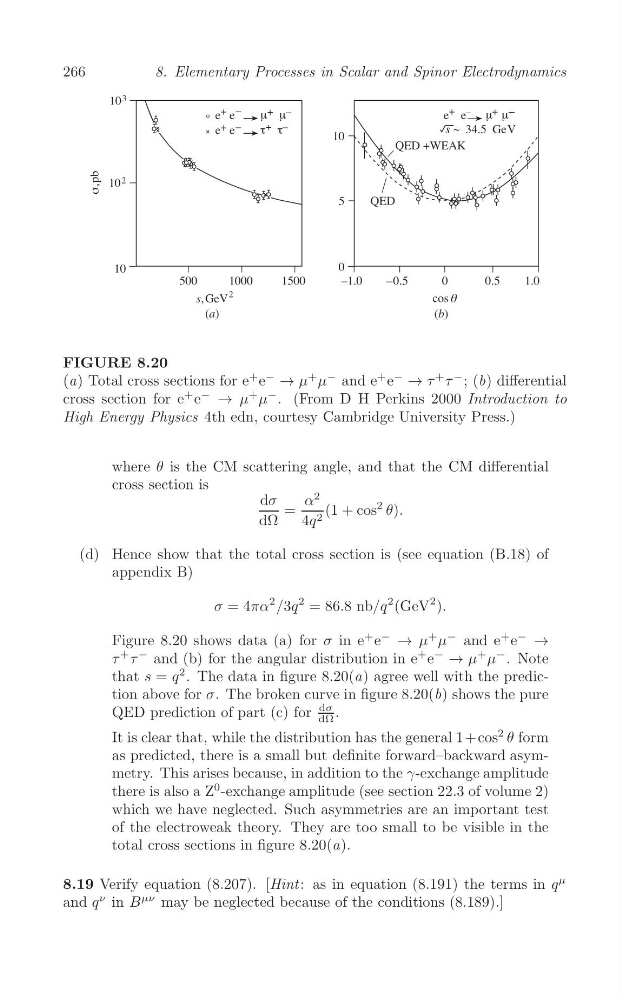
FIGURE 8.20
+
(a) Total cross sections for e
+ e
−
→ μ
+ μ
− and e e
−
→ τ
+ τ
− ; (b) differential
−
→ μ
+ μ
−
cross section for e
+ e
. (From D H Perkins 2000 Introduction to
High Energy Physics 4th edn, courtesy Cambridge University Press.)
where θ is the CM scattering angle, and that the CM differential
cross section is
dσ
α
2
=
(1 + cos
2 θ).
dΩ
4q 2
(d) Hence show that the total cross section is (see equation (B.18) of
appendix B)
σ = 4πα
2 /3q
2 = 86.8 nb/q
2 (GeV
2 ).
−
→ μ
+ μ
−
−
Figure 8.20 shows data (a) for σ in e
+ e
and e
+ e →
τ
+ τ
− and (b) for the angular distribution in e
+ e
−
→ μ
+ μ
− . Note
that s = q
2 . The data in figure 8.20(a) agree well with the prediction above for σ. The broken curve in figure 8.20(b) shows the pure
QED prediction of part (c) for
dσ
dΩ .
It is clear that, while the distribution has the general 1+cos
2 θ form
as predicted, there is a small but definite forward–backward asymmetry. This arises because, in addition to the γ-exchange amplitude
there is also a Z
0 -exchange amplitude (see section 22.3 of volume 2)
which we have neglected. Such asymmetries are an important test
of the electroweak theory. They are too small to be visible in the
total cross sections in figure 8.20(a).
μ
8.19 Verify equation (8.207). [Hint : as in equation (8.191) the terms in q
ν
and q in B
μν may be neglected because of the conditions (8.189).]
8. Elementary Processes in Scalar and Spinor Electrodynamics
FIGURE 8.20
+
(a) Total cross sections for e
+ e
−
→ μ
+ μ
− and e e
−
→ τ
+ τ
− ; (b) differential
−
→ μ
+ μ
−
cross section for e
+ e
. (From D H Perkins 2000 Introduction to
High Energy Physics 4th edn, courtesy Cambridge University Press.)
where θ is the CM scattering angle, and that the CM differential
cross section is
dσ
α
2
=
(1 + cos
2 θ).
dΩ
4q 2
(d) Hence show that the total cross section is (see equation (B.18) of
appendix B)
σ = 4πα
2 /3q
2 = 86.8 nb/q
2 (GeV
2 ).
−
→ μ
+ μ
−
−
Figure 8.20 shows data (a) for σ in e
+ e
and e
+ e →
τ
+ τ
− and (b) for the angular distribution in e
+ e
−
→ μ
+ μ
− . Note
that s = q
2 . The data in figure 8.20(a) agree well with the prediction above for σ. The broken curve in figure 8.20(b) shows the pure
QED prediction of part (c) for
dσ
dΩ .
It is clear that, while the distribution has the general 1+cos
2 θ form
as predicted, there is a small but definite forward–backward asymmetry. This arises because, in addition to the γ-exchange amplitude
there is also a Z
0 -exchange amplitude (see section 22.3 of volume 2)
which we have neglected. Such asymmetries are an important test
of the electroweak theory. They are too small to be visible in the
total cross sections in figure 8.20(a).
μ
8.19 Verify equation (8.207). [Hint : as in equation (8.191) the terms in q
ν
and q in B
μν may be neglected because of the conditions (8.189).]