

262
8. Elementary Processes in Scalar and Spinor Electrodynamics
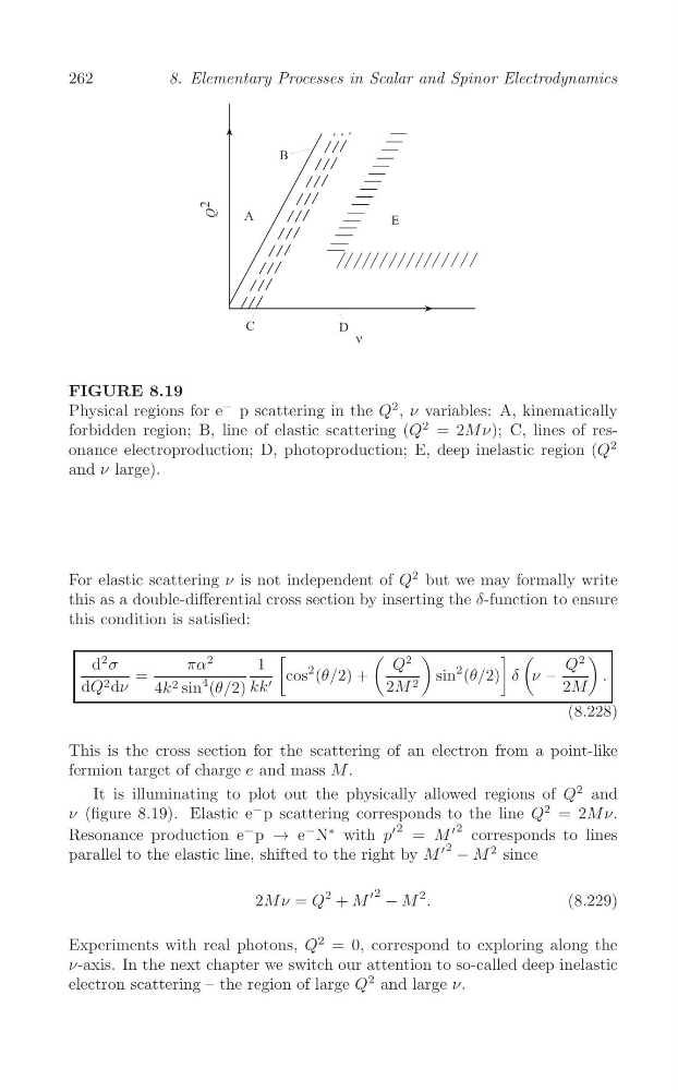
FIGURE 8.19
Physical regions for e
− p scattering in the Q
2 , ν variables: A, kinematically
forbidden region; B, line of elastic scattering (Q
2 = 2M ν); C, lines of resonance electroproduction; D, photoproduction; E, deep inelastic region (Q
2
and ν large).
For elastic scattering ν is not independent of Q
2 but we may formally write
this as a double-differential cross section by inserting the δ-function to ensure
this condition is satisfied:
[
(
)
] (
)
d
2 σ
πα
2
1
Q
2
Q
2
=
cos
2 (θ/2) +
sin
2 (θ/2) δ ν −
.
dQ 2 dν
4k 2 sin
4 (θ/2) kk ′
2M 2
2M
(8.228)
This is the cross section for the scattering of an electron from a point-like
fermion target of charge e and mass M .
It is illuminating to plot out the physically allowed regions of Q
2 and
ν (figure 8.19). Elastic e
− p scattering corresponds to the line Q
2 = 2M ν.
′ 2
′ 2
Resonance production e
− p → e
− N
∗ with p = M corresponds to lines
parallel to the elastic line, shifted to the right by M
′ 2 − M
2 since
′ 2
Q
2
− M
2
2M ν =
+ M
.
(8.229)
Experiments with real photons, Q
2 = 0, correspond to exploring along the
ν-axis. In the next chapter we switch our attention to so-called deep inelastic
electron scattering – the region of large Q
2 and large ν.
8. Elementary Processes in Scalar and Spinor Electrodynamics
FIGURE 8.19
Physical regions for e
− p scattering in the Q
2 , ν variables: A, kinematically
forbidden region; B, line of elastic scattering (Q
2 = 2M ν); C, lines of resonance electroproduction; D, photoproduction; E, deep inelastic region (Q
2
and ν large).
For elastic scattering ν is not independent of Q
2 but we may formally write
this as a double-differential cross section by inserting the δ-function to ensure
this condition is satisfied:
[
(
)
] (
)
d
2 σ
πα
2
1
Q
2
Q
2
=
cos
2 (θ/2) +
sin
2 (θ/2) δ ν −
.
dQ 2 dν
4k 2 sin
4 (θ/2) kk ′
2M 2
2M
(8.228)
This is the cross section for the scattering of an electron from a point-like
fermion target of charge e and mass M .
It is illuminating to plot out the physically allowed regions of Q
2 and
ν (figure 8.19). Elastic e
− p scattering corresponds to the line Q
2 = 2M ν.
′ 2
′ 2
Resonance production e
− p → e
− N
∗ with p = M corresponds to lines
parallel to the elastic line, shifted to the right by M
′ 2 − M
2 since
′ 2
Q
2
− M
2
2M ν =
+ M
.
(8.229)
Experiments with real photons, Q
2 = 0, correspond to exploring along the
ν-axis. In the next chapter we switch our attention to so-called deep inelastic
electron scattering – the region of large Q
2 and large ν.