

229
8.2. Coulomb scattering of charged spin1 particles
2
of the scattered electron and are not sensitive to the spin state s
′ . Thus what
we wish to calculate, in this case, is the unpolarized cross section defined by
d¯ σ ≡
1 (dσ ↑↑ + dσ ↑↓ + dσ ↓↑ + dσ ↓↓ )
2 ∑
1
=
dσ s ' s
(8.45)
2
s ' ,s
2
where dσ s ' ,s ∝ |u
† (k
′ , s
′ )u(k, s)| . In (8.45), we are averaging over the two
possible initial spin polarizations and summing over the final spin states arising
from each initial spin state.
It is possible to calculate the quantity
∑
1
′ † 2
S =
|u u|
(8.46)
2
'
s ,s
by brute force, using (3.73) and taking the two-component spinors to be, say,
( )
( )
1
0
φ
1 =
φ
2 =
.
(8.47)
0
1
One finds (problem 8.4)
S = (2E)
2 (1 − v
2 sin
2 θ/2)
(8.48)
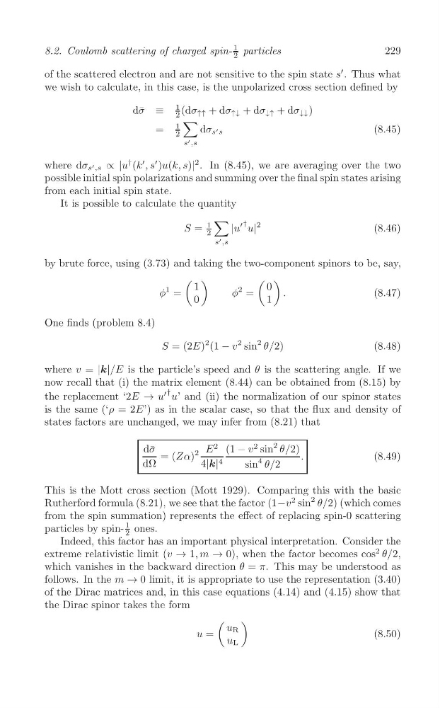
where v = |k|/E is the particle’s speed and θ is the scattering angle. If we
now recall that (i) the matrix element (8.44) can be obtained from (8.15) by
′ †
the replacement ‘2E → u u’ and (ii) the normalization of our spinor states
is the same (‘ρ = 2E’) as in the scalar case, so that the flux and density of
states factors are unchanged, we may infer from (8.21) that
d¯ σ
E
2 (1 − v
2 sin
2 θ/2)
= (Zα)
2
.
(8.49)
4
dΩ
4|k|
sin
4 θ/2
This is the Mott cross section (Mott 1929). Comparing this with the basic
Rutherford formula (8.21), we see that the factor (1−v
2 sin
2 θ/2) (which comes
from the spin summation) represents the effect of replacing spin-0 scattering
particles by spin1 ones.
2
Indeed, this factor has an important physical interpretation. Consider the
extreme relativistic limit (v → 1, m → 0), when the factor becomes cos
2 θ/2,
which vanishes in the backward direction θ = π. This may be understood as
follows. In the m → 0 limit, it is appropriate to use the representation (3.40)
of the Dirac matrices and, in this case equations (4.14) and (4.15) show that
the Dirac spinor takes the form
(
)
u R
u =
(8.50)
u L
8.2. Coulomb scattering of charged spin1 particles
2
of the scattered electron and are not sensitive to the spin state s
′ . Thus what
we wish to calculate, in this case, is the unpolarized cross section defined by
d¯ σ ≡
1 (dσ ↑↑ + dσ ↑↓ + dσ ↓↑ + dσ ↓↓ )
2 ∑
1
=
dσ s ' s
(8.45)
2
s ' ,s
2
where dσ s ' ,s ∝ |u
† (k
′ , s
′ )u(k, s)| . In (8.45), we are averaging over the two
possible initial spin polarizations and summing over the final spin states arising
from each initial spin state.
It is possible to calculate the quantity
∑
1
′ † 2
S =
|u u|
(8.46)
2
'
s ,s
by brute force, using (3.73) and taking the two-component spinors to be, say,
( )
( )
1
0
φ
1 =
φ
2 =
.
(8.47)
0
1
One finds (problem 8.4)
S = (2E)
2 (1 − v
2 sin
2 θ/2)
(8.48)
where v = |k|/E is the particle’s speed and θ is the scattering angle. If we
now recall that (i) the matrix element (8.44) can be obtained from (8.15) by
′ †
the replacement ‘2E → u u’ and (ii) the normalization of our spinor states
is the same (‘ρ = 2E’) as in the scalar case, so that the flux and density of
states factors are unchanged, we may infer from (8.21) that
d¯ σ
E
2 (1 − v
2 sin
2 θ/2)
= (Zα)
2
.
(8.49)
4
dΩ
4|k|
sin
4 θ/2
This is the Mott cross section (Mott 1929). Comparing this with the basic
Rutherford formula (8.21), we see that the factor (1−v
2 sin
2 θ/2) (which comes
from the spin summation) represents the effect of replacing spin-0 scattering
particles by spin1 ones.
2
Indeed, this factor has an important physical interpretation. Consider the
extreme relativistic limit (v → 1, m → 0), when the factor becomes cos
2 θ/2,
which vanishes in the backward direction θ = π. This may be understood as
follows. In the m → 0 limit, it is appropriate to use the representation (3.40)
of the Dirac matrices and, in this case equations (4.14) and (4.15) show that
the Dirac spinor takes the form
(
)
u R
u =
(8.50)
u L