

224
8. Elementary Processes in Scalar and Spinor Electrodynamics
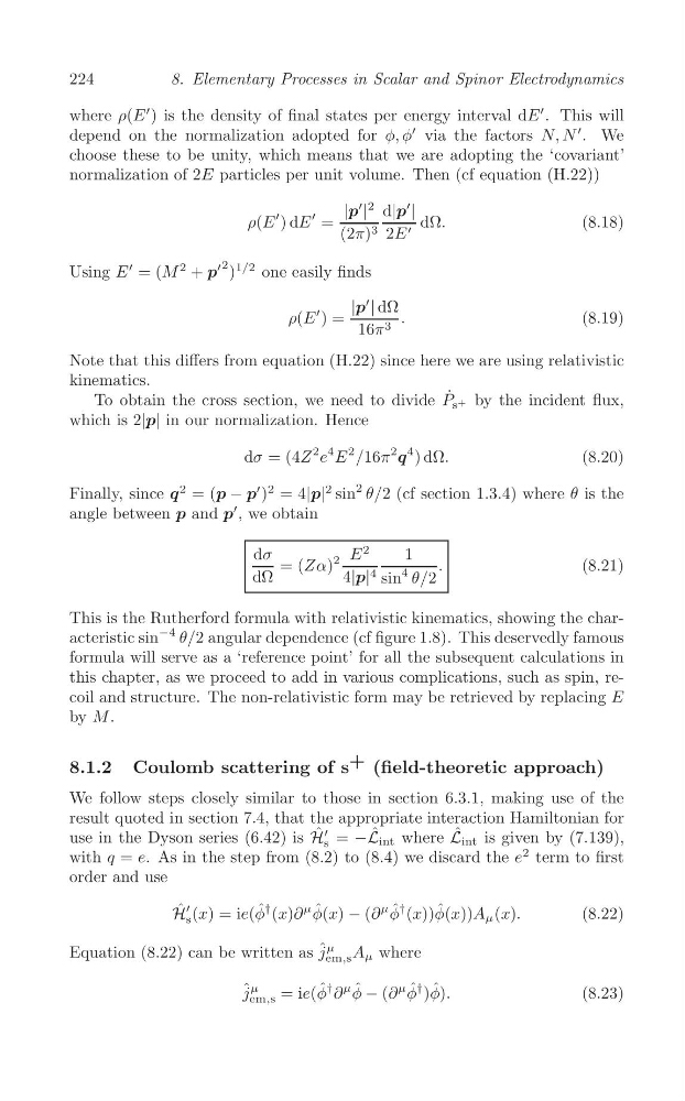
where ρ(E
′ ) is the density of final states per energy interval dE
′ . This will
depend on the normalization adopted for φ, φ
′ via the factors N, N
′ . We
choose these to be unity, which means that we are adopting the ‘covariant’
normalization of 2E particles per unit volume. Then (cf equation (H.22))
′
|
2
|p d|p
′
|
ρ(E
′ ) dE
′ =
dΩ.
(8.18)
(2π) 3 2E ′
′ 2 )
1/2
Using E
′ = (M
2 + p
one easily finds
|p
′
| dΩ
ρ(E
′ ) =
.
(8.19)
16π 3
Note that this differs from equation (H.22) since here we are using relativistic
kinematics.
To obtain the cross section, we need to divide P ˙ s + by the incident flux,
which is 2|p| in our normalization. Hence
dσ = (4Z
2 e
4 E
2 /16π
2
q
4 ) dΩ.
(8.20)
Finally, since q
2 = (p − p
′ )
2 = 4|p|
2 sin
2 θ/2 (cf section 1.3.4) where θ is the
angle between p and p
′ , we obtain
E
2
dσ = (Zα)
2
1
.
(8.21)
dΩ
4|p| 4 sin
4 θ/2
This is the Rutherford formula with relativistic kinematics, showing the characteristic sin
−4 θ/2 angular dependence (cf figure 1.8). This deservedly famous
formula will serve as a ‘reference point’ for all the subsequent calculations in
this chapter, as we proceed to add in various complications, such as spin, recoil and structure. The non-relativistic form may be retrieved by replacing E
by M .
8.1.2 Coulomb scattering of s + (field-theoretic approach)
We follow steps closely similar to those in section 6.3.1, making use of the
result quoted in section 7.4, that the appropriate interaction Hamiltonian for
use in the Dyson series (6.42) is H ˆ
s
′ = −L ˆ int where L ˆ int is given by (7.139),
2
with q = e. As in the step from (8.2) to (8.4) we discard the e term to first
order and use
H ˆ ′ (x) = ie(φ ˆ † (x)∂
μ φ ˆ (x) − (∂
μ φ ˆ † (x))φ ˆ (x))A μ (x).
(8.22)
s
Equation (8.22) can be written as ˆ j
μ
A μ where
em,s
ˆ j
μ
= ie(φ ˆ † ∂
μ φ ˆ − (∂
μ φ ˆ † )φ ˆ ).
(8.23)
em,s
8. Elementary Processes in Scalar and Spinor Electrodynamics
where ρ(E
′ ) is the density of final states per energy interval dE
′ . This will
depend on the normalization adopted for φ, φ
′ via the factors N, N
′ . We
choose these to be unity, which means that we are adopting the ‘covariant’
normalization of 2E particles per unit volume. Then (cf equation (H.22))
′
|
2
|p d|p
′
|
ρ(E
′ ) dE
′ =
dΩ.
(8.18)
(2π) 3 2E ′
′ 2 )
1/2
Using E
′ = (M
2 + p
one easily finds
|p
′
| dΩ
ρ(E
′ ) =
.
(8.19)
16π 3
Note that this differs from equation (H.22) since here we are using relativistic
kinematics.
To obtain the cross section, we need to divide P ˙ s + by the incident flux,
which is 2|p| in our normalization. Hence
dσ = (4Z
2 e
4 E
2 /16π
2
q
4 ) dΩ.
(8.20)
Finally, since q
2 = (p − p
′ )
2 = 4|p|
2 sin
2 θ/2 (cf section 1.3.4) where θ is the
angle between p and p
′ , we obtain
E
2
dσ = (Zα)
2
1
.
(8.21)
dΩ
4|p| 4 sin
4 θ/2
This is the Rutherford formula with relativistic kinematics, showing the characteristic sin
−4 θ/2 angular dependence (cf figure 1.8). This deservedly famous
formula will serve as a ‘reference point’ for all the subsequent calculations in
this chapter, as we proceed to add in various complications, such as spin, recoil and structure. The non-relativistic form may be retrieved by replacing E
by M .
8.1.2 Coulomb scattering of s + (field-theoretic approach)
We follow steps closely similar to those in section 6.3.1, making use of the
result quoted in section 7.4, that the appropriate interaction Hamiltonian for
use in the Dyson series (6.42) is H ˆ
s
′ = −L ˆ int where L ˆ int is given by (7.139),
2
with q = e. As in the step from (8.2) to (8.4) we discard the e term to first
order and use
H ˆ ′ (x) = ie(φ ˆ † (x)∂
μ φ ˆ (x) − (∂
μ φ ˆ † (x))φ ˆ (x))A μ (x).
(8.22)
s
Equation (8.22) can be written as ˆ j
μ
A μ where
em,s
ˆ j
μ
= ie(φ ˆ † ∂
μ φ ˆ − (∂
μ φ ˆ † )φ ˆ ).
(8.23)
em,s