

202
7. Quantum Field Theory III
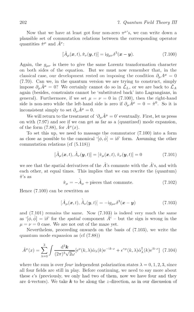
Now that we have at least got four non-zero π
μ ’s, we can write down a
plausible set of commutation relations between the corresponding operator
quantities ˆ
π
μ and A ˆ ν :
[A ˆ μ (x, t), π ˆ ν (y, t)] = ig μν δ
3 (x − y).
(7.100)
Again, the g μν is there to give the same Lorentz transformation character
on both sides of the equation. But we must now remember that, in the
classical case, our development rested on imposing the condition ∂ μ A
μ = 0
(7.70). Can we, in the quantum version we are trying to construct, simply
impose ∂ μ A ˆ μ = 0? We certainly cannot do so in L ˆ L , or we are back to L ˆ A
again (besides, constraints cannot be ‘substituted back’ into Lagrangians, in
general). Furthermore, if we set μ = ν = 0 in (7.100), then the right-hand
A ˆ μ
side is non-zero while the left-hand side is zero if ∂ μ
= 0 = ˆ
π
0 . So it is
inconsistent simply to set ∂ μ A ˆ μ = 0.
A ˆ μ
We will return to the treatment of ‘∂ μ
= 0’ eventually. First, let us press
on with (7.97) and see if we can get as far as a (quantized) mode expansion,
of the form (7.88), for A ˆ μ (x).
To set this up, we need to massage the commutator (7.100) into a form
as close as possible to the canonical ‘[φ, φ ˙ ] = iδ’ form. Assuming the other
commutation relations (cf (5.118))
[A ˆ μ (x, t), A ˆ ν (y, t)] = [ˆ π μ (x, t), π ˆ ν (y, t)] = 0
(7.101)
we see that the spatial derivatives of the A ˆ ’s commute with the A ˆ ’s, and with
each other, at equal times. This implies that we can rewrite the (quantum)
π ˆ’s as
˙ ˆ
π ˆ μ = −A μ + pieces that commute.
(7.102)
Hence (7.100) can be rewritten as
[A ˆ μ (x, t), A
˙ ˆ ν (y, t)] = −ig μν δ
3 (x − y)
(7.103)
and (7.101) remains the same. Now (7.103) is indeed very much the same
as ‘[φ, φ ˙ ] = iδ’ for the spatial component A ˆ i – but the sign is wrong in the
μ = ν = 0 case. We are not out of the maze yet.
Nevertheless, proceeding onwards on the basis of (7.103), we write the
quantum mode expansion as (cf (7.88))
3 ∫
∑
d
3
k
†
A ˆ μ (x) =
√ [∈
μ (k, λ)ˆ α λ (k)e
−ik·x + ∈
∗μ (k, λ)ˆ α (k)e
ik·x ] (7.104)
λ
(2π) 3 2ω
λ=0
where the sum is over four independent polarization states λ = 0, 1, 2, 3, since
all four fields are still in play. Before continuing, we need to say more about
these ∈’s (previously, we only had two of them, now we have four and they
are 4-vectors). We take k to be along the z-direction, as in our discussion of
7. Quantum Field Theory III
Now that we have at least got four non-zero π
μ ’s, we can write down a
plausible set of commutation relations between the corresponding operator
quantities ˆ
π
μ and A ˆ ν :
[A ˆ μ (x, t), π ˆ ν (y, t)] = ig μν δ
3 (x − y).
(7.100)
Again, the g μν is there to give the same Lorentz transformation character
on both sides of the equation. But we must now remember that, in the
classical case, our development rested on imposing the condition ∂ μ A
μ = 0
(7.70). Can we, in the quantum version we are trying to construct, simply
impose ∂ μ A ˆ μ = 0? We certainly cannot do so in L ˆ L , or we are back to L ˆ A
again (besides, constraints cannot be ‘substituted back’ into Lagrangians, in
general). Furthermore, if we set μ = ν = 0 in (7.100), then the right-hand
A ˆ μ
side is non-zero while the left-hand side is zero if ∂ μ
= 0 = ˆ
π
0 . So it is
inconsistent simply to set ∂ μ A ˆ μ = 0.
A ˆ μ
We will return to the treatment of ‘∂ μ
= 0’ eventually. First, let us press
on with (7.97) and see if we can get as far as a (quantized) mode expansion,
of the form (7.88), for A ˆ μ (x).
To set this up, we need to massage the commutator (7.100) into a form
as close as possible to the canonical ‘[φ, φ ˙ ] = iδ’ form. Assuming the other
commutation relations (cf (5.118))
[A ˆ μ (x, t), A ˆ ν (y, t)] = [ˆ π μ (x, t), π ˆ ν (y, t)] = 0
(7.101)
we see that the spatial derivatives of the A ˆ ’s commute with the A ˆ ’s, and with
each other, at equal times. This implies that we can rewrite the (quantum)
π ˆ’s as
˙ ˆ
π ˆ μ = −A μ + pieces that commute.
(7.102)
Hence (7.100) can be rewritten as
[A ˆ μ (x, t), A
˙ ˆ ν (y, t)] = −ig μν δ
3 (x − y)
(7.103)
and (7.101) remains the same. Now (7.103) is indeed very much the same
as ‘[φ, φ ˙ ] = iδ’ for the spatial component A ˆ i – but the sign is wrong in the
μ = ν = 0 case. We are not out of the maze yet.
Nevertheless, proceeding onwards on the basis of (7.103), we write the
quantum mode expansion as (cf (7.88))
3 ∫
∑
d
3
k
†
A ˆ μ (x) =
√ [∈
μ (k, λ)ˆ α λ (k)e
−ik·x + ∈
∗μ (k, λ)ˆ α (k)e
ik·x ] (7.104)
λ
(2π) 3 2ω
λ=0
where the sum is over four independent polarization states λ = 0, 1, 2, 3, since
all four fields are still in play. Before continuing, we need to say more about
these ∈’s (previously, we only had two of them, now we have four and they
are 4-vectors). We take k to be along the z-direction, as in our discussion of