

195
7.2. The Dirac field and the spin-statistics connection
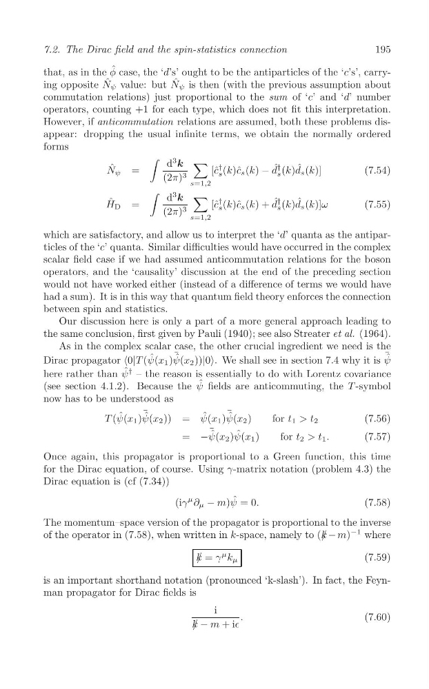
that, as in the φ ˆ case, the ‘d’s’ ought to be the antiparticles of the ‘c’s’, carrying opposite N ˆ ψ value: but N ˆ ψ is then (with the previous assumption about
commutation relations) just proportional to the sum of ‘c’ and ‘d’ number
operators, counting +1 for each type, which does not fit this interpretation.
However, if anticommutation relations are assumed, both these problems disappear: dropping the usual infinite terms, we obtain the normally ordered
forms
∫ d
3
k ∑ †
†
N ˆ ψ =
[ˆ c (k)ˆ c s (k) − d ˆ (k)d ˆ s (k)]
(7.54)
s
s
(2π) 3
s=1,2
∫ d
3
k ∑ †
†
H ˆ D =
[ˆ c s (k)ˆ c s (k) + d ˆ (k)d ˆ s (k)]ω
(7.55)
s
(2π) 3
s=1,2
which are satisfactory, and allow us to interpret the ‘d’ quanta as the antiparticles of the ‘c’ quanta. Similar difficulties would have occurred in the complex
scalar field case if we had assumed anticommutation relations for the boson
operators, and the ‘causality’ discussion at the end of the preceding section
would not have worked either (instead of a difference of terms we would have
had a sum). It is in this way that quantum field theory enforces the connection
between spin and statistics.
Our discussion here is only a part of a more general approach leading to
the same conclusion, first given by Pauli (1940); see also Streater et al. (1964).
As in the complex scalar case, the other crucial ingredient we need is the
¯ ˆ
¯ ˆ
Dirac propagator <0|T (ψ ˆ (x 1 )ψ(x 2 ))|0>. We shall see in section 7.4 why it is ψ
†
here rather than ψ ˆ – the reason is essentially to do with Lorentz covariance
(see section 4.1.2). Because the ψ ˆ fields are anticommuting, the T -symbol
now has to be understood as
¯
¯
T ( ˆ
ˆ
ˆ
ˆ
ψ(x 1 )ψ(x 2 )) = ψ(x 1 )ψ(x 2 )
for t 1 > t 2
(7.56)
¯
= −ψ ˆ (x 2 )ψ ˆ (x 1 )
for t 2 > t 1 .
(7.57)
Once again, this propagator is proportional to a Green function, this time
for the Dirac equation, of course. Using γ-matrix notation (problem 4.3) the
Dirac equation is (cf (7.34))
(iγ
μ ∂ μ − m)ψ ˆ = 0.
(7.58)
The momentum–space version of the propagator is proportional to the inverse
of the operator in (7.58), when written in k-space, namely to (k / − m)
−1 where
k / = γ
μ k μ
(7.59)
is an important shorthand notation (pronounced ‘k-slash’). In fact, the Feynman propagator for Dirac fields is
i
.
(7.60)
k / − m + i∈
7.2. The Dirac field and the spin-statistics connection
that, as in the φ ˆ case, the ‘d’s’ ought to be the antiparticles of the ‘c’s’, carrying opposite N ˆ ψ value: but N ˆ ψ is then (with the previous assumption about
commutation relations) just proportional to the sum of ‘c’ and ‘d’ number
operators, counting +1 for each type, which does not fit this interpretation.
However, if anticommutation relations are assumed, both these problems disappear: dropping the usual infinite terms, we obtain the normally ordered
forms
∫ d
3
k ∑ †
†
N ˆ ψ =
[ˆ c (k)ˆ c s (k) − d ˆ (k)d ˆ s (k)]
(7.54)
s
s
(2π) 3
s=1,2
∫ d
3
k ∑ †
†
H ˆ D =
[ˆ c s (k)ˆ c s (k) + d ˆ (k)d ˆ s (k)]ω
(7.55)
s
(2π) 3
s=1,2
which are satisfactory, and allow us to interpret the ‘d’ quanta as the antiparticles of the ‘c’ quanta. Similar difficulties would have occurred in the complex
scalar field case if we had assumed anticommutation relations for the boson
operators, and the ‘causality’ discussion at the end of the preceding section
would not have worked either (instead of a difference of terms we would have
had a sum). It is in this way that quantum field theory enforces the connection
between spin and statistics.
Our discussion here is only a part of a more general approach leading to
the same conclusion, first given by Pauli (1940); see also Streater et al. (1964).
As in the complex scalar case, the other crucial ingredient we need is the
¯ ˆ
¯ ˆ
Dirac propagator <0|T (ψ ˆ (x 1 )ψ(x 2 ))|0>. We shall see in section 7.4 why it is ψ
†
here rather than ψ ˆ – the reason is essentially to do with Lorentz covariance
(see section 4.1.2). Because the ψ ˆ fields are anticommuting, the T -symbol
now has to be understood as
¯
¯
T ( ˆ
ˆ
ˆ
ˆ
ψ(x 1 )ψ(x 2 )) = ψ(x 1 )ψ(x 2 )
for t 1 > t 2
(7.56)
¯
= −ψ ˆ (x 2 )ψ ˆ (x 1 )
for t 2 > t 1 .
(7.57)
Once again, this propagator is proportional to a Green function, this time
for the Dirac equation, of course. Using γ-matrix notation (problem 4.3) the
Dirac equation is (cf (7.34))
(iγ
μ ∂ μ − m)ψ ˆ = 0.
(7.58)
The momentum–space version of the propagator is proportional to the inverse
of the operator in (7.58), when written in k-space, namely to (k / − m)
−1 where
k / = γ
μ k μ
(7.59)
is an important shorthand notation (pronounced ‘k-slash’). In fact, the Feynman propagator for Dirac fields is
i
.
(7.60)
k / − m + i∈