

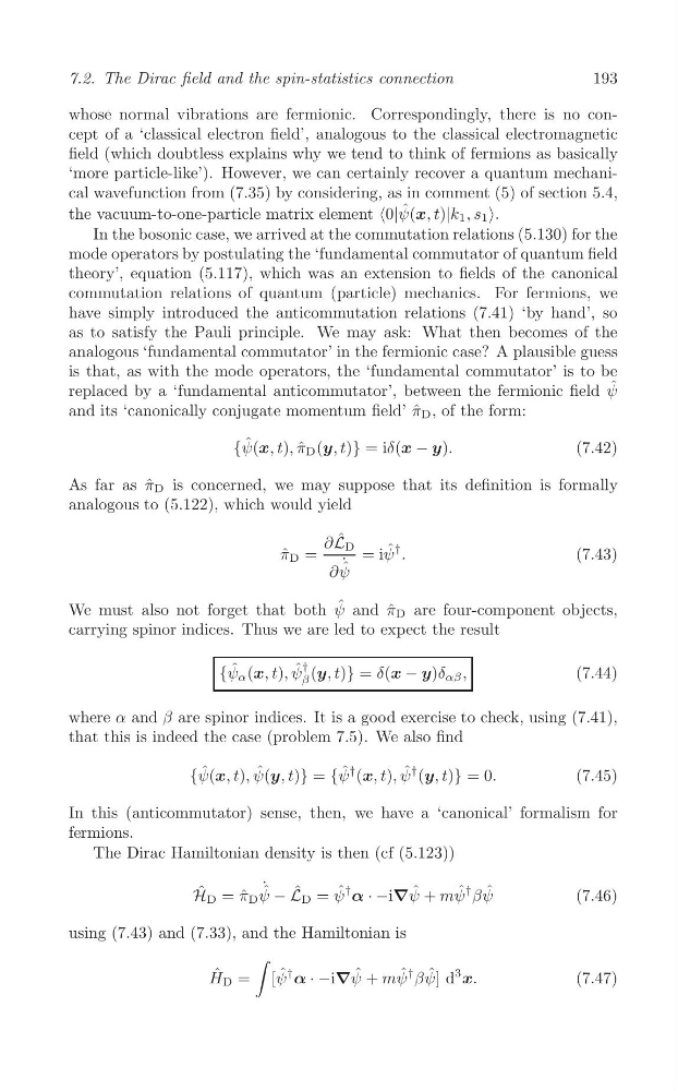
193
7.2. The Dirac field and the spin-statistics connection
whose normal vibrations are fermionic. Correspondingly, there is no concept of a ‘classical electron field’, analogous to the classical electromagnetic
field (which doubtless explains why we tend to think of fermions as basically
‘more particle-like’). However, we can certainly recover a quantum mechanical wavefunction from (7.35) by considering, as in comment (5) of section 5.4,
the vacuum-to-one-particle matrix element <0|ψ ˆ (x, t)|k 1 , s 1 >.
In the bosonic case, we arrived at the commutation relations (5.130) for the
mode operators by postulating the ‘fundamental commutator of quantum field
theory’, equation (5.117), which was an extension to fields of the canonical
commutation relations of quantum (particle) mechanics. For fermions, we
have simply introduced the anticommutation relations (7.41) ‘by hand’, so
as to satisfy the Pauli principle. We may ask: What then becomes of the
analogous ‘fundamental commutator’ in the fermionic case? A plausible guess
is that, as with the mode operators, the ‘fundamental commutator’ is to be
replaced by a ‘fundamental anticommutator’, between the fermionic field ψ ˆ
and its ‘canonically conjugate momentum field’ π ˆ D , of the form:
{ψ ˆ (x, t), π ˆ D (y, t)} = iδ(x − y).
(7.42)
As far as ˆ
π D is concerned, we may suppose that its definition is formally
analogous to (5.122), which would yield
∂ ˆ
L D
ψ
†
π ˆ D =
= i ˆ .
(7.43)
˙ ˆ
∂ψ
We must also not forget that both ψ ˆ and ˆ
π D are four-component objects,
carrying spinor indices. Thus we are led to expect the result
{ψ ˆ α (x, t), ψ ˆ
β
† (y, t)} = δ(x − y)δ αβ ,
(7.44)
where α and β are spinor indices. It is a good exercise to check, using (7.41),
that this is indeed the case (problem 7.5). We also find
{ψ ˆ (x, t), ψ ˆ (y, t)} = {ψ ˆ † (x, t), ψ ˆ † (y, t)} = 0.
(7.45)
In this (anticommutator) sense, then, we have a ‘canonical’ formalism for
fermions.
The Dirac Hamiltonian density is then (cf (5.123))
H ˆ D = ˆ
π D ψ
˙ ˆ − L ˆ D = ψ ˆ † α · −i∇ψ ˆ + mψ ˆ † βψ ˆ
(7.46)
using (7.43) and (7.33), and the Hamiltonian is
∫
H ˆ D = [ψ ˆ † α · −i∇ψ ˆ + mψ ˆ † βψ ˆ ] d
3
x.
(7.47)
7.2. The Dirac field and the spin-statistics connection
whose normal vibrations are fermionic. Correspondingly, there is no concept of a ‘classical electron field’, analogous to the classical electromagnetic
field (which doubtless explains why we tend to think of fermions as basically
‘more particle-like’). However, we can certainly recover a quantum mechanical wavefunction from (7.35) by considering, as in comment (5) of section 5.4,
the vacuum-to-one-particle matrix element <0|ψ ˆ (x, t)|k 1 , s 1 >.
In the bosonic case, we arrived at the commutation relations (5.130) for the
mode operators by postulating the ‘fundamental commutator of quantum field
theory’, equation (5.117), which was an extension to fields of the canonical
commutation relations of quantum (particle) mechanics. For fermions, we
have simply introduced the anticommutation relations (7.41) ‘by hand’, so
as to satisfy the Pauli principle. We may ask: What then becomes of the
analogous ‘fundamental commutator’ in the fermionic case? A plausible guess
is that, as with the mode operators, the ‘fundamental commutator’ is to be
replaced by a ‘fundamental anticommutator’, between the fermionic field ψ ˆ
and its ‘canonically conjugate momentum field’ π ˆ D , of the form:
{ψ ˆ (x, t), π ˆ D (y, t)} = iδ(x − y).
(7.42)
As far as ˆ
π D is concerned, we may suppose that its definition is formally
analogous to (5.122), which would yield
∂ ˆ
L D
ψ
†
π ˆ D =
= i ˆ .
(7.43)
˙ ˆ
∂ψ
We must also not forget that both ψ ˆ and ˆ
π D are four-component objects,
carrying spinor indices. Thus we are led to expect the result
{ψ ˆ α (x, t), ψ ˆ
β
† (y, t)} = δ(x − y)δ αβ ,
(7.44)
where α and β are spinor indices. It is a good exercise to check, using (7.41),
that this is indeed the case (problem 7.5). We also find
{ψ ˆ (x, t), ψ ˆ (y, t)} = {ψ ˆ † (x, t), ψ ˆ † (y, t)} = 0.
(7.45)
In this (anticommutator) sense, then, we have a ‘canonical’ formalism for
fermions.
The Dirac Hamiltonian density is then (cf (5.123))
H ˆ D = ˆ
π D ψ
˙ ˆ − L ˆ D = ψ ˆ † α · −i∇ψ ˆ + mψ ˆ † βψ ˆ
(7.46)
using (7.43) and (7.33), and the Hamiltonian is
∫
H ˆ D = [ψ ˆ † α · −i∇ψ ˆ + mψ ˆ † βψ ˆ ] d
3
x.
(7.47)