

153
6.2. Perturbation theory for interacting fields
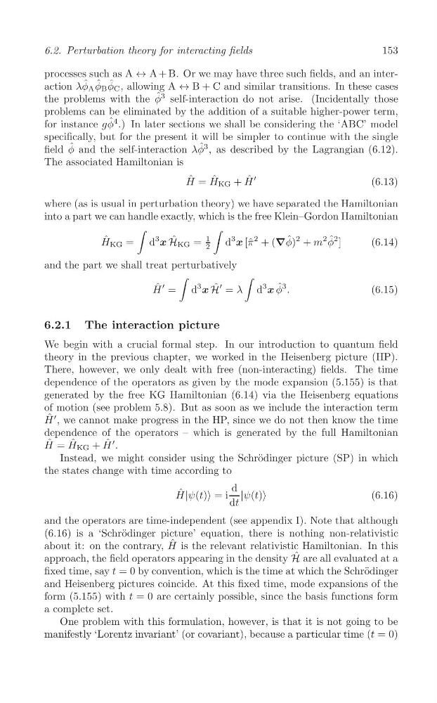
processes such as A ↔ A + B. Or we may have three such fields, and an interaction λφ ˆ A φ ˆ B φ ˆ C , allowing A ↔ B + C and similar transitions. In these cases
the problems with the φ ˆ3 self-interaction do not arise. (Incidentally those
problems can be eliminated by the addition of a suitable higher-power term,
for instance gφ ˆ 4 .) In later sections we shall be considering the ‘ABC’ model
specifically, but for the present it will be simpler to continue with the single
field φ ˆ and the self-interaction λφ ˆ3 , as described by the Lagrangian (6.12).
The associated Hamiltonian is
′
H ˆ = H ˆ KG + H ˆ
(6.13)
where (as is usual in perturbation theory) we have separated the Hamiltonian
into a part we can handle exactly, which is the free Klein–Gordon Hamiltonian
∫
∫
H ˆ KG = d
3
x H ˆ KG =
1
d
3
x [ˆ π
2 + (∇φ ˆ )
2 + m
2 φ ˆ 2 ]
(6.14)
2
and the part we shall treat perturbatively
∫
∫
H ˆ ′ = d
3
x H ˆ ′ = λ d
3
x φ ˆ 3 .
(6.15)
6.2.1 The interaction picture
We begin with a crucial formal step. In our introduction to quantum field
theory in the previous chapter, we worked in the Heisenberg picture (HP).
There, however, we only dealt with free (non-interacting) fields. The time
dependence of the operators as given by the mode expansion (5.155) is that
generated by the free KG Hamiltonian (6.14) via the Heisenberg equations
of motion (see problem 5.8). But as soon as we include the interaction term
H ˆ ′ , we cannot make progress in the HP, since we do not then know the time
dependence of the operators – which is generated by the full Hamiltonian
ˆ H ˆ KG + ˆ ′
H =
H .
Instead, we might consider using the Schr¨ odinger picture (SP) in which
the states change with time according to
d
ˆ
H|ψ(t)> = i |ψ(t)>
(6.16)
dt
and the operators are time-independent (see appendix I). Note that although
(6.16) is a ‘Schr¨ odinger picture’ equation, there is nothing non-relativistic
about it: on the contrary, H ˆ is the relevant relativistic Hamiltonian. In this
approach, the field operators appearing in the density H ˆ are all evaluated at a
fixed time, say t = 0 by convention, which is the time at which the Schr¨ odinger
and Heisenberg pictures coincide. At this fixed time, mode expansions of the
form (5.155) with t = 0 are certainly possible, since the basis functions form
a complete set.
One problem with this formulation, however, is that it is not going to be
manifestly ‘Lorentz invariant’ (or covariant), because a particular time (t = 0)
6.2. Perturbation theory for interacting fields
processes such as A ↔ A + B. Or we may have three such fields, and an interaction λφ ˆ A φ ˆ B φ ˆ C , allowing A ↔ B + C and similar transitions. In these cases
the problems with the φ ˆ3 self-interaction do not arise. (Incidentally those
problems can be eliminated by the addition of a suitable higher-power term,
for instance gφ ˆ 4 .) In later sections we shall be considering the ‘ABC’ model
specifically, but for the present it will be simpler to continue with the single
field φ ˆ and the self-interaction λφ ˆ3 , as described by the Lagrangian (6.12).
The associated Hamiltonian is
′
H ˆ = H ˆ KG + H ˆ
(6.13)
where (as is usual in perturbation theory) we have separated the Hamiltonian
into a part we can handle exactly, which is the free Klein–Gordon Hamiltonian
∫
∫
H ˆ KG = d
3
x H ˆ KG =
1
d
3
x [ˆ π
2 + (∇φ ˆ )
2 + m
2 φ ˆ 2 ]
(6.14)
2
and the part we shall treat perturbatively
∫
∫
H ˆ ′ = d
3
x H ˆ ′ = λ d
3
x φ ˆ 3 .
(6.15)
6.2.1 The interaction picture
We begin with a crucial formal step. In our introduction to quantum field
theory in the previous chapter, we worked in the Heisenberg picture (HP).
There, however, we only dealt with free (non-interacting) fields. The time
dependence of the operators as given by the mode expansion (5.155) is that
generated by the free KG Hamiltonian (6.14) via the Heisenberg equations
of motion (see problem 5.8). But as soon as we include the interaction term
H ˆ ′ , we cannot make progress in the HP, since we do not then know the time
dependence of the operators – which is generated by the full Hamiltonian
ˆ H ˆ KG + ˆ ′
H =
H .
Instead, we might consider using the Schr¨ odinger picture (SP) in which
the states change with time according to
d
ˆ
H|ψ(t)> = i |ψ(t)>
(6.16)
dt
and the operators are time-independent (see appendix I). Note that although
(6.16) is a ‘Schr¨ odinger picture’ equation, there is nothing non-relativistic
about it: on the contrary, H ˆ is the relevant relativistic Hamiltonian. In this
approach, the field operators appearing in the density H ˆ are all evaluated at a
fixed time, say t = 0 by convention, which is the time at which the Schr¨ odinger
and Heisenberg pictures coincide. At this fixed time, mode expansions of the
form (5.155) with t = 0 are certainly possible, since the basis functions form
a complete set.
One problem with this formulation, however, is that it is not going to be
manifestly ‘Lorentz invariant’ (or covariant), because a particular time (t = 0)