

150
6. Quantum Field Theory II: Interacting Scalar Fields
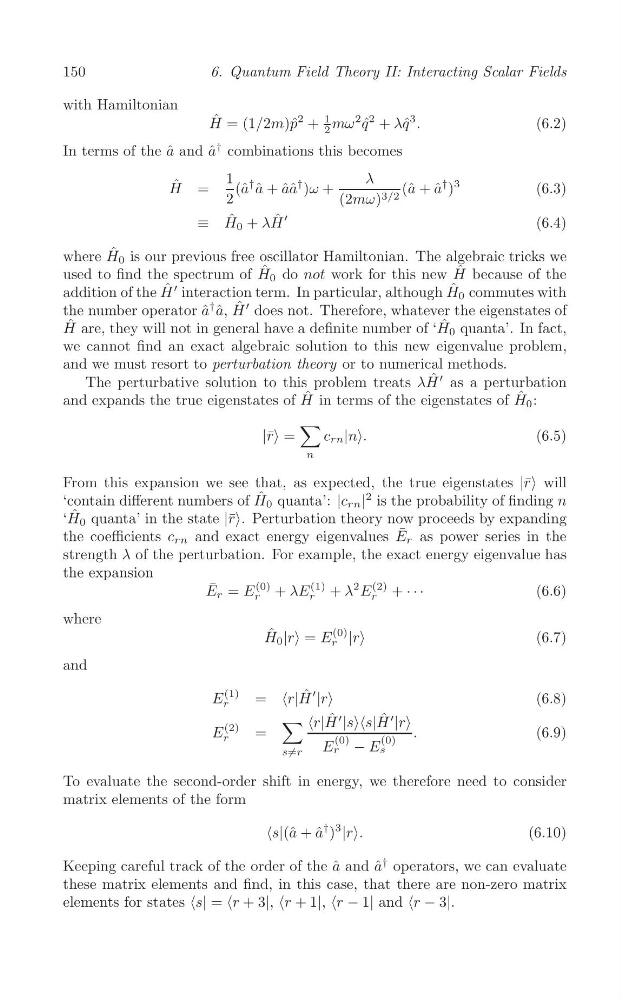
with Hamiltonian
ˆ
2
1
2
3
H = (1/2m)ˆ p + mω
2 q ˆ + λq ˆ .
(6.2)
2
In terms of the ˆ
a and ˆ
a
† combinations this becomes
ˆ
1 † ˆ
λ
† )
3
H =
(ˆ a a + ˆ
aa ˆ
† )ω +
(ˆ a + ˆ
a
(6.3)
2
(2mω) 3/2
′
≡ H ˆ 0 + λH ˆ
(6.4)
where H ˆ 0 is our previous free oscillator Hamiltonian. The algebraic tricks we
used to find the spectrum of H ˆ 0 do not work for this new H ˆ because of the
′
addition of the H ˆ interaction term. In particular, although H ˆ 0 commutes with
the number operator a ˆ
† a ˆ, H ˆ ′ does not. Therefore, whatever the eigenstates of
ˆ
ˆ
H are, they will not in general have a definite number of ‘H 0 quanta’. In fact,
we cannot find an exact algebraic solution to this new eigenvalue problem,
and we must resort to perturbation theory or to numerical methods.
′
The perturbative solution to this problem treats λH ˆ as a perturbation
and expands the true eigenstates of H ˆ in terms of the eigenstates of H ˆ 0 :
∑
|r ¯> =
c rn |n>.
(6.5)
n
From this expansion we see that, as expected, the true eigenstates |r ¯> will
‘contain different numbers of H ˆ 0 quanta’: |c rn |
2 is the probability of finding n
ˆ
‘H 0 quanta’ in the state |r ¯>. Perturbation theory now proceeds by expanding
the coefficients c rn and exact energy eigenvalues E ¯ r as power series in the
strength λ of the perturbation. For example, the exact energy eigenvalue has
the expansion
¯
E
(0) + λE
(1) + λ
2 E
(2)
E r =
r
+ · · ·
(6.6)
r
r
where
ˆ
E
(0)
H 0 |r> =
|r>
(6.7)
r
and
E
(1) =
(6.8)
r
∑
E
(2) =
.
(6.9)
r
(0)
(0)
s/
E r − E s
=r
To evaluate the second-order shift in energy, we therefore need to consider
matrix elements of the form
† )
3
|r>.
(6.10)
Keeping careful track of the order of the ˆ
a and ˆ
a
† operators, we can evaluate
these matrix elements and find, in this case, that there are non-zero matrix
elements for states
6. Quantum Field Theory II: Interacting Scalar Fields
with Hamiltonian
ˆ
2
1
2
3
H = (1/2m)ˆ p + mω
2 q ˆ + λq ˆ .
(6.2)
2
In terms of the ˆ
a and ˆ
a
† combinations this becomes
ˆ
1 † ˆ
λ
† )
3
H =
(ˆ a a + ˆ
aa ˆ
† )ω +
(ˆ a + ˆ
a
(6.3)
2
(2mω) 3/2
′
≡ H ˆ 0 + λH ˆ
(6.4)
where H ˆ 0 is our previous free oscillator Hamiltonian. The algebraic tricks we
used to find the spectrum of H ˆ 0 do not work for this new H ˆ because of the
′
addition of the H ˆ interaction term. In particular, although H ˆ 0 commutes with
the number operator a ˆ
† a ˆ, H ˆ ′ does not. Therefore, whatever the eigenstates of
ˆ
ˆ
H are, they will not in general have a definite number of ‘H 0 quanta’. In fact,
we cannot find an exact algebraic solution to this new eigenvalue problem,
and we must resort to perturbation theory or to numerical methods.
′
The perturbative solution to this problem treats λH ˆ as a perturbation
and expands the true eigenstates of H ˆ in terms of the eigenstates of H ˆ 0 :
∑
|r ¯> =
c rn |n>.
(6.5)
n
From this expansion we see that, as expected, the true eigenstates |r ¯> will
‘contain different numbers of H ˆ 0 quanta’: |c rn |
2 is the probability of finding n
ˆ
‘H 0 quanta’ in the state |r ¯>. Perturbation theory now proceeds by expanding
the coefficients c rn and exact energy eigenvalues E ¯ r as power series in the
strength λ of the perturbation. For example, the exact energy eigenvalue has
the expansion
¯
E
(0) + λE
(1) + λ
2 E
(2)
E r =
r
+ · · ·
(6.6)
r
r
where
ˆ
E
(0)
H 0 |r> =
|r>
(6.7)
r
and
E
(1) =
(6.8)
r
∑
E
(2) =
.
(6.9)
r
(0)
(0)
s/
E r − E s
=r
To evaluate the second-order shift in energy, we therefore need to consider
matrix elements of the form
† )
3
|r>.
(6.10)
Keeping careful track of the order of the ˆ
a and ˆ
a
† operators, we can evaluate
these matrix elements and find, in this case, that there are non-zero matrix
elements for states