

136
5. Quantum Field Theory I: The Free Scalar Field
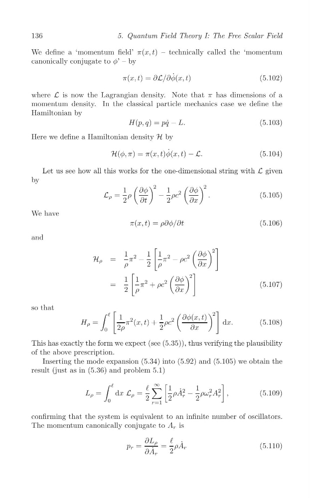
We define a ‘momentum field’ π(x, t) – technically called the ‘momentum
canonically conjugate to φ’ – by
π(x, t) = ∂L/∂φ ˙ (x, t)
(5.102)
where L is now the Lagrangian density. Note that π has dimensions of a
momentum density. In the classical particle mechanics case we define the
Hamiltonian by
H(p, q) = pq˙ − L.
(5.103)
Here we define a Hamiltonian density H by
H(φ, π) = π(x, t)φ ˙ (x, t) − L.
(5.104)
Let us see how all this works for the one-dimensional string with L given
by
( ) 2
( ) 2
1
∂φ
1
∂φ
L ρ = ρ
− ρc
2
.
(5.105)
2
∂t
2
∂x
We have
π(x, t) = ρ∂φ/∂t
(5.106)
and
[
( ) 2
]
1
1 1
∂φ
H ρ =
π
2
−
π
2
− ρc
2
ρ
2 ρ
∂x
[
( ) 2
]
1 1
∂φ
π
2
2 ρ
∂x
=
+ ρc
2
(5.107)
so that
∫ [
(
) 2
]
e
1
1
∂φ(x, t)
H ρ =
π
2 (x, t) + ρc
2
dx.
(5.108)
0
2ρ
2
∂x
This has exactly the form we expect (see (5.35)), thus verifying the plausibility
of the above prescription.
Inserting the mode expansion (5.34) into (5.92) and (5.105) we obtain the
result (just as in (5.36) and problem 5.1)
∫
[
]
e
∞
∑
e
1
1
L ρ =
dx L ρ =
ρA ˙
r
2
− ρω
2 A r
2 ,
(5.109)
r
2
2
2
0
r=1
confirming that the system is equivalent to an infinite number of oscillators.
The momentum canonically conjugate to A r is
∂L ρ
e
p r =
= ρA ˙ r
(5.110)
∂A ˙ r
2
5. Quantum Field Theory I: The Free Scalar Field
We define a ‘momentum field’ π(x, t) – technically called the ‘momentum
canonically conjugate to φ’ – by
π(x, t) = ∂L/∂φ ˙ (x, t)
(5.102)
where L is now the Lagrangian density. Note that π has dimensions of a
momentum density. In the classical particle mechanics case we define the
Hamiltonian by
H(p, q) = pq˙ − L.
(5.103)
Here we define a Hamiltonian density H by
H(φ, π) = π(x, t)φ ˙ (x, t) − L.
(5.104)
Let us see how all this works for the one-dimensional string with L given
by
( ) 2
( ) 2
1
∂φ
1
∂φ
L ρ = ρ
− ρc
2
.
(5.105)
2
∂t
2
∂x
We have
π(x, t) = ρ∂φ/∂t
(5.106)
and
[
( ) 2
]
1
1 1
∂φ
H ρ =
π
2
−
π
2
− ρc
2
ρ
2 ρ
∂x
[
( ) 2
]
1 1
∂φ
π
2
2 ρ
∂x
=
+ ρc
2
(5.107)
so that
∫ [
(
) 2
]
e
1
1
∂φ(x, t)
H ρ =
π
2 (x, t) + ρc
2
dx.
(5.108)
0
2ρ
2
∂x
This has exactly the form we expect (see (5.35)), thus verifying the plausibility
of the above prescription.
Inserting the mode expansion (5.34) into (5.92) and (5.105) we obtain the
result (just as in (5.36) and problem 5.1)
∫
[
]
e
∞
∑
e
1
1
L ρ =
dx L ρ =
ρA ˙
r
2
− ρω
2 A r
2 ,
(5.109)
r
2
2
2
0
r=1
confirming that the system is equivalent to an infinite number of oscillators.
The momentum canonically conjugate to A r is
∂L ρ
e
p r =
= ρA ˙ r
(5.110)
∂A ˙ r
2