

134
5. Quantum Field Theory I: The Free Scalar Field
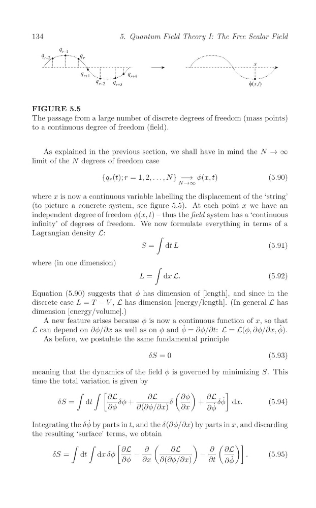
FIGURE 5.5
The passage from a large number of discrete degrees of freedom (mass points)
to a continuous degree of freedom (field).
As explained in the previous section, we shall have in mind the N → ∞
limit of the N degrees of freedom case
{q r (t); r = 1, 2, . . . , N} −→ φ(x, t)
(5.90)
N →∞
where x is now a continuous variable labelling the displacement of the ‘string’
(to picture a concrete system, see figure 5.5). At each point x we have an
independent degree of freedom φ(x, t) – thus the field system has a ‘continuous
infinity’ of degrees of freedom. We now formulate everything in terms of a
Lagrangian density L:
∫
S = dt L
(5.91)
where (in one dimension)
∫
L = dx L.
(5.92)
Equation (5.90) suggests that φ has dimension of [length], and since in the
discrete case L = T − V , L has dimension [energy/length]. (In general L has
dimension [energy/volume].)
A new feature arises because φ is now a continuous function of x, so that
L can depend on ∂φ/∂x as well as on φ and φ ˙ = ∂φ/∂t: L = L(φ, ∂φ/∂x, φ ˙ ).
As before, we postulate the same fundamental principle
δS = 0
(5.93)
meaning that the dynamics of the field φ is governed by minimizing S. This
time the total variation is given by
∫
∫ [
( )
]
∂L
∂L
∂φ
∂L
δS = dt
δφ +
δ
+
δφ ˙ dx.
(5.94)
∂φ
∂(∂φ/∂x)
∂x
∂φ ˙
Integrating the δφ ˙ by parts in t, and the δ(∂φ/∂x) by parts in x, and discarding
the resulting ‘surface’ terms, we obtain
∫
∫
[
(
)
(
)]
∂L
∂
∂L
∂ ∂L
δS = dt dx δφ
−
−
.
(5.95)
∂φ
∂x ∂(∂φ/∂x)
∂t ∂φ ˙
5. Quantum Field Theory I: The Free Scalar Field
FIGURE 5.5
The passage from a large number of discrete degrees of freedom (mass points)
to a continuous degree of freedom (field).
As explained in the previous section, we shall have in mind the N → ∞
limit of the N degrees of freedom case
{q r (t); r = 1, 2, . . . , N} −→ φ(x, t)
(5.90)
N →∞
where x is now a continuous variable labelling the displacement of the ‘string’
(to picture a concrete system, see figure 5.5). At each point x we have an
independent degree of freedom φ(x, t) – thus the field system has a ‘continuous
infinity’ of degrees of freedom. We now formulate everything in terms of a
Lagrangian density L:
∫
S = dt L
(5.91)
where (in one dimension)
∫
L = dx L.
(5.92)
Equation (5.90) suggests that φ has dimension of [length], and since in the
discrete case L = T − V , L has dimension [energy/length]. (In general L has
dimension [energy/volume].)
A new feature arises because φ is now a continuous function of x, so that
L can depend on ∂φ/∂x as well as on φ and φ ˙ = ∂φ/∂t: L = L(φ, ∂φ/∂x, φ ˙ ).
As before, we postulate the same fundamental principle
δS = 0
(5.93)
meaning that the dynamics of the field φ is governed by minimizing S. This
time the total variation is given by
∫
∫ [
( )
]
∂L
∂L
∂φ
∂L
δS = dt
δφ +
δ
+
δφ ˙ dx.
(5.94)
∂φ
∂(∂φ/∂x)
∂x
∂φ ˙
Integrating the δφ ˙ by parts in t, and the δ(∂φ/∂x) by parts in x, and discarding
the resulting ‘surface’ terms, we obtain
∫
∫
[
(
)
(
)]
∂L
∂
∂L
∂ ∂L
δS = dt dx δφ
−
−
.
(5.95)
∂φ
∂x ∂(∂φ/∂x)
∂t ∂φ ˙