

98
4. Lorentz Transformations and Discrete Symmetries
0
the reader may check in problem 4.4(a) that v is a scalar and v is a polar
vector.
More interesting possibilities emerge when we introduce a new γ-matrix,
γ 5 , defined by
γ 5 = iγ
0 γ
1 γ
2 γ
3 .
(4.77)
This matrix has the defining property that it anticommutes with the γ
μ matrices:
{γ 5 , γ
μ
} = 0.
(4.78)
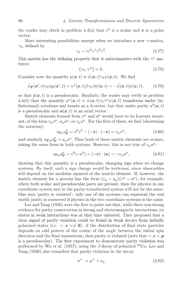
Consider now the quantity p(x, t) ≡ ψ ¯ (x, t)γ 5 ψ(x, t). We find
¯
′
′
¯
ψ P (x , t)γ 5 ψ P (x , t) = ψ
† (x, t)βγ 5 βψ(x, t) = −ψ(x, t)ψ(x, t),
(4.79)
so that p(x, t) is a pseudoscalar. Similarly, the reader may verify in problem
4.4(b) that the quantity a
μ (x, t) ≡ ψ ¯ (x, t)γ 5 γ
μ ψ(x, t) transforms under (infinitesimal) rotations and boosts as a 4-vector, but that under parity a
0 (x, t)
is a pseudoscalar and a(x, t) is an axial vector.
Matrix elements formed from v
μ and a
μ would have to be Lorentz invariμ
μ
ant, of the form v μ v , a μ a , or v μ a
μ . For the first of these, we find (shortening
the notation)
μ
0
μ
v Pμ v = v v
0
− (−v) · (−v) = v μ v ,
(4.80)
P
μ
μ
and similarly a Pμ a P = a μ a . Thus both of these matrix elements are scalars,
μ
taking the same form in both systems. However, this is not true of v μ a :
μ
μ
v Pμ a = v
0 (−a
0 ) − (−v) · (a) = −v μ a ,
(4.81)
P
showing that this quantity is a pseudoscalar, changing sign when we change
systems. By itself, such a sign change would be irrelevant, since observables
will depend on the modulus squared of the matrix element. If, however, the
matrix element for a process has the form (v μ − a μ )(v
μ
− a
μ ), for example,
where both scalar and pseudoscalar parts are present, then the physics in one
coordinate system and in the parity-transformed system will not be the same.
One says ‘parity is violated’: only one of the systems can represent the real
world; parity is conserved if physics in the two coordinate systems is the same.
Lee and Yang (1956) were the first to point out that, while there was strong
evidence for parity conservation in strong and electromagnetic interactions, its
status in weak interactions was at that time untested. They proposed that a
clear signal of parity violation could be found in weak decays from initially
polarized states (i.e. < s >/ = 0): if the distribution of final state particles
depends on odd powers of the cosine of the angle between the initial spin
direction and the final momentum, then parity is violated (note that < s > ·p
is a pseudoscalar). The first experiment to demonstrate parity violation was
performed by Wu et al. (1957), using the β-decay of polarized
60 Co. Lee and
Yang (1956) also remarked that parity violation in the decay
π
+
→ μ
+ + ν μ
(4.82)
4. Lorentz Transformations and Discrete Symmetries
0
the reader may check in problem 4.4(a) that v is a scalar and v is a polar
vector.
More interesting possibilities emerge when we introduce a new γ-matrix,
γ 5 , defined by
γ 5 = iγ
0 γ
1 γ
2 γ
3 .
(4.77)
This matrix has the defining property that it anticommutes with the γ
μ matrices:
{γ 5 , γ
μ
} = 0.
(4.78)
Consider now the quantity p(x, t) ≡ ψ ¯ (x, t)γ 5 ψ(x, t). We find
¯
′
′
¯
ψ P (x , t)γ 5 ψ P (x , t) = ψ
† (x, t)βγ 5 βψ(x, t) = −ψ(x, t)ψ(x, t),
(4.79)
so that p(x, t) is a pseudoscalar. Similarly, the reader may verify in problem
4.4(b) that the quantity a
μ (x, t) ≡ ψ ¯ (x, t)γ 5 γ
μ ψ(x, t) transforms under (infinitesimal) rotations and boosts as a 4-vector, but that under parity a
0 (x, t)
is a pseudoscalar and a(x, t) is an axial vector.
Matrix elements formed from v
μ and a
μ would have to be Lorentz invariμ
μ
ant, of the form v μ v , a μ a , or v μ a
μ . For the first of these, we find (shortening
the notation)
μ
0
μ
v Pμ v = v v
0
− (−v) · (−v) = v μ v ,
(4.80)
P
μ
μ
and similarly a Pμ a P = a μ a . Thus both of these matrix elements are scalars,
μ
taking the same form in both systems. However, this is not true of v μ a :
μ
μ
v Pμ a = v
0 (−a
0 ) − (−v) · (a) = −v μ a ,
(4.81)
P
showing that this quantity is a pseudoscalar, changing sign when we change
systems. By itself, such a sign change would be irrelevant, since observables
will depend on the modulus squared of the matrix element. If, however, the
matrix element for a process has the form (v μ − a μ )(v
μ
− a
μ ), for example,
where both scalar and pseudoscalar parts are present, then the physics in one
coordinate system and in the parity-transformed system will not be the same.
One says ‘parity is violated’: only one of the systems can represent the real
world; parity is conserved if physics in the two coordinate systems is the same.
Lee and Yang (1956) were the first to point out that, while there was strong
evidence for parity conservation in strong and electromagnetic interactions, its
status in weak interactions was at that time untested. They proposed that a
clear signal of parity violation could be found in weak decays from initially
polarized states (i.e. < s >/ = 0): if the distribution of final state particles
depends on odd powers of the cosine of the angle between the initial spin
direction and the final momentum, then parity is violated (note that < s > ·p
is a pseudoscalar). The first experiment to demonstrate parity violation was
performed by Wu et al. (1957), using the β-decay of polarized
60 Co. Lee and
Yang (1956) also remarked that parity violation in the decay
π
+
→ μ
+ + ν μ
(4.82)