

Data Reduction
25
57,213 - 62,073
t=
I-1 1"]
1/2
t = -0.3380
-9(29,287)2 + 9(28,223)211/2
30,505 cycles
(1.86)
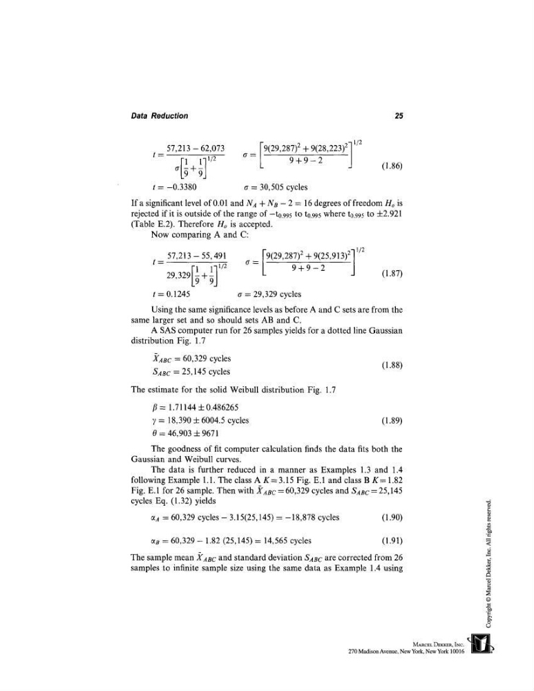
Ifa significant level of 0.01 and N~ + NB - 2 = 16 degrees of freedom Ho is
rejected if it is outside of the range of -t0.995 to t0.995 where t0.995 to 4-2.921
(Table E.2). Therefore Ho is accepted.
Now comparing A and C:
57,213 - 55,491
29,329[~ + ~]
1/2
0.1245
a = [9(29’287)2 + 9(q5’913)2"] ~/2 L ~
29,329 cycles
(1.87)
1.71144 4- 0.486265
18,390 4- 6004.5 cycles
(1.89)
46,903 + 9671
goodness of fit computer calculation finds the data fits both the
and Weibull curves.
data is further reduced in a manner as Examples 1.3 and 1.4
Using the same significance levels as before A and C sets are from the
same larger set and so should sets AB and C.
A SAS computer run for 26 samples yields for a dotted line Gaussian
distribution Fig. 1.7
~(nBc = 60,329 cycles
S.4~c = 25,145 cycles
(1.88)
The estimate for the solid Weibull distribution Fig. 1.7
0=
The
Gaussian
The
following Example 1.1. The class A K=3.15 Fig. E.1 and class B K= 1.82
Fig. E. 1 for 26 sample. Then with ~A~c = 60,329 cycles and Sa~c = 25,145
cycles Eq. (1.32) yields
an = 60,329 cycles - 3.15(25,145) = -18,878 cycles
(1.90)
c~ = 60,329- 1.82 (25,145)= 14,565 cycles
(1.91)
The sample mean X~c and standard deviation SaBc are corrected from 26
samples to infinite sample size using the same data as Example 1.4 using
25
57,213 - 62,073
t=
I-1 1"]
1/2
t = -0.3380
-9(29,287)2 + 9(28,223)211/2
30,505 cycles
(1.86)
Ifa significant level of 0.01 and N~ + NB - 2 = 16 degrees of freedom Ho is
rejected if it is outside of the range of -t0.995 to t0.995 where t0.995 to 4-2.921
(Table E.2). Therefore Ho is accepted.
Now comparing A and C:
57,213 - 55,491
29,329[~ + ~]
1/2
0.1245
a = [9(29’287)2 + 9(q5’913)2"] ~/2 L ~
29,329 cycles
(1.87)
1.71144 4- 0.486265
18,390 4- 6004.5 cycles
(1.89)
46,903 + 9671
goodness of fit computer calculation finds the data fits both the
and Weibull curves.
data is further reduced in a manner as Examples 1.3 and 1.4
Using the same significance levels as before A and C sets are from the
same larger set and so should sets AB and C.
A SAS computer run for 26 samples yields for a dotted line Gaussian
distribution Fig. 1.7
~(nBc = 60,329 cycles
S.4~c = 25,145 cycles
(1.88)
The estimate for the solid Weibull distribution Fig. 1.7
0=
The
Gaussian
The
following Example 1.1. The class A K=3.15 Fig. E.1 and class B K= 1.82
Fig. E. 1 for 26 sample. Then with ~A~c = 60,329 cycles and Sa~c = 25,145
cycles Eq. (1.32) yields
an = 60,329 cycles - 3.15(25,145) = -18,878 cycles
(1.90)
c~ = 60,329- 1.82 (25,145)= 14,565 cycles
(1.91)
The sample mean X~c and standard deviation SaBc are corrected from 26
samples to infinite sample size using the same data as Example 1.4 using