14
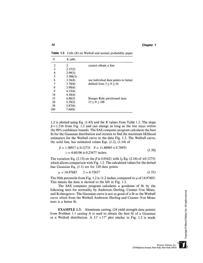
Table 1.3 Cells (K) on Weibull and normal probability paper
Chapter 1
N
K cells
2
2
cannot obtain a line
3
2.57(3)
4
2.99(3)
5
3.306(3)
6
3.56(4)
use individual data points to better
7
3.78(4)
defined lines 3 < N < 10
8
3.98(4)
9
4.15(4)
10
4.30(4)
15
4.88(5)
Sturges Rule partitioned data
20
5.29(5)
15 < N< 100
30
5.87(6)
100
7.60(8)
1.2 is plotted using Eq. (1.43) and the K values from Table 1.2. The slope
/3--1.516 from Fig. 1.2 and can change as long as the line stays within
the 90% confidence bounds. The SAS computer program calculates the best
fit for the Gaussian distribution and iterates to find the maximum liklihood
estimaters for the Weibull curve to the data Fig. 1.3. The Weibull curve,
the solid line, has estimated values Eqs. (1.2), (1.14)
/~=1.589174-0.12731
0=11.48905+0.76931
7 = 4.68106 4- 0.23477 inches
(1.50)
The variation Eq. (2.13) on the/~ is 0.01621 with ~# Eq. (2.16) of +0.12731
which allows comparison with Fig. 1.2. The calculated values for the dotted
line Gaussian Eq. (1.1) are for 120 data points
/~ = 14.97683
} = 6.72417
(1.51)
The 50th percentile from Fig. 1.2 is 11.2 inches, compared to # of 14.97683.
This means the data is skewed to the left in Fig. 1.3.
The SAS computer program calculates a goodness of fit by the
following tests for normality by Anderson-Darling, Cramer-Von Mises,
and Kolmogorov. The Gaussian curve is not as good of a fit as the Weibull
curve which from the Weibull Anderson-Darling and Cramer-Von Mises
tests is a better fit.
EXAMPLE 1.3. Aluminum casting, (24 yield strength data points)
from Problem 1.1 casting A is used to obtain the best fit of a Gaussian
or a Weibull distribution. A ll"x 17" plot similar to Fig. 1.2 is made