

224
Appendix A
Further noting fl ranges from about 1 to higher values most generally
around 5-10 for a Gaussian distribution.
In all forms by definition
normalized
R(t) + Q(t) -- 1
(A.8)
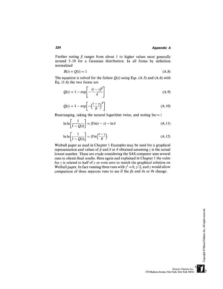
The equation is solved for the failure Q(t) using Eqs. (A.5) and (A.6)
Eq. (1.4) the two forms are
Q(t)= 1-exp ¯
(A.9)
In ln[1 _~l~(t)] = flln(t - ~) -
lnln[1
_~] = ~ ln(~)
(A.11)
(A.12)
Weibull paper as used in Chapter 1 Examples may be used for a graphical
representation and values of fl and 6 or 0 obtained assuming y is the actual
lowest number. These are crude considering the SAS computer uses several
runs to obtain final results. Here again and explained in Chapter 1 the value
for ~ is related to half of ~ or even zero to match the graphical solution on
Weibull paper. In fact running three runs with 71 = 0, y/2, and y would allow
comparison of three separate runs to see if the fls and 6s or 0s change.
Q(t) = 1 - exp -
(A. 10)
Rearranging, taking the natural logarithm twice, and noting lne = 1
Appendix A
Further noting fl ranges from about 1 to higher values most generally
around 5-10 for a Gaussian distribution.
In all forms by definition
normalized
R(t) + Q(t) -- 1
(A.8)
The equation is solved for the failure Q(t) using Eqs. (A.5) and (A.6)
Eq. (1.4) the two forms are
Q(t)= 1-exp ¯
(A.9)
In ln[1 _~l~(t)] = flln(t - ~) -
lnln[1
_~] = ~ ln(~)
(A.11)
(A.12)
Weibull paper as used in Chapter 1 Examples may be used for a graphical
representation and values of fl and 6 or 0 obtained assuming y is the actual
lowest number. These are crude considering the SAS computer uses several
runs to obtain final results. Here again and explained in Chapter 1 the value
for ~ is related to half of ~ or even zero to match the graphical solution on
Weibull paper. In fact running three runs with 71 = 0, y/2, and y would allow
comparison of three separate runs to see if the fls and 6s or 0s change.
Q(t) = 1 - exp -
(A. 10)
Rearranging, taking the natural logarithm twice, and noting lne = 1