

192
Chapter 4
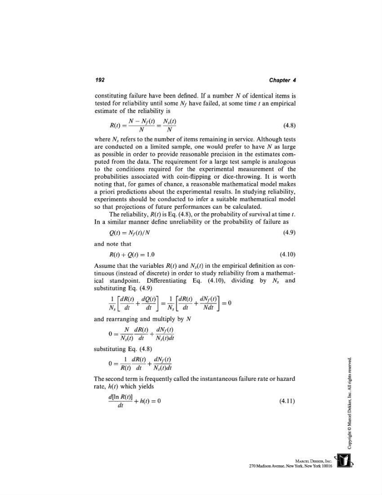
constituting failure have been defined. If a number N of identical items is
tested for reliability until some Nf have failed, at some time t an empirical
estimate of the reliability is
R(t) - N Nf(t) _ Ns(t~)
(4.8)
N
N
where Ns refers to the number of items remaining in service. Although tests
are conducted on a limited sample, one would prefer to have N as large
as possible in order to provide reasonable precision in the estimates computed from the data. The requirement for a large test sample is analogous
to the conditions required for the experimental measurement of the
probabilities associated with coin-flipping or dice-throwing. It is worth
noting that, for games of chance, a reasonable mathematical model makes
a priori predictions about the experimental results. In studying reliability,
experiments should be conducted to infer a suitable mathematical model
so that projections of future performances can be calculated.
The reliability, R(t) is Eq. (4.8), or the probability of survival at time
In a similar manner ’define unreliability or the probability of failure as
Q(t) = Nf(t)/N
(4.9)
and note that
R(t) + Q(t) = 1.0
(4.10)
Assume that the variables R(t) and Ns(t) in the empirical definition as continuous (instead of discrete) in order to study reliability from a mathematical standpoint.
Differentiating
Eq. (4.10), dividing by Ns and
substituting Eq. (4.9)
1 FdR(t ) dQ(t)l 1 [dR(t) dNf(t)]
~ssL dt + dt J =-~sL dt + Ndt J =0
and rearranging and multiply by N
dNf(t)
o - N~ ~lR(t~) +-Ns(t) dt N~(t)dt
substituting Eq. (4.8)
dNf(t)
o - ~ ~(t~ + ~
R(t) dt NAt)dt
The second term is frequently called the instantaneous failure rate or hazard
rate, h(t) which yields
a[~n g(0]
~ +~(t) =
(4.~)
dt
Chapter 4
constituting failure have been defined. If a number N of identical items is
tested for reliability until some Nf have failed, at some time t an empirical
estimate of the reliability is
R(t) - N Nf(t) _ Ns(t~)
(4.8)
N
N
where Ns refers to the number of items remaining in service. Although tests
are conducted on a limited sample, one would prefer to have N as large
as possible in order to provide reasonable precision in the estimates computed from the data. The requirement for a large test sample is analogous
to the conditions required for the experimental measurement of the
probabilities associated with coin-flipping or dice-throwing. It is worth
noting that, for games of chance, a reasonable mathematical model makes
a priori predictions about the experimental results. In studying reliability,
experiments should be conducted to infer a suitable mathematical model
so that projections of future performances can be calculated.
The reliability, R(t) is Eq. (4.8), or the probability of survival at time
In a similar manner ’define unreliability or the probability of failure as
Q(t) = Nf(t)/N
(4.9)
and note that
R(t) + Q(t) = 1.0
(4.10)
Assume that the variables R(t) and Ns(t) in the empirical definition as continuous (instead of discrete) in order to study reliability from a mathematical standpoint.
Differentiating
Eq. (4.10), dividing by Ns and
substituting Eq. (4.9)
1 FdR(t ) dQ(t)l 1 [dR(t) dNf(t)]
~ssL dt + dt J =-~sL dt + Ndt J =0
and rearranging and multiply by N
dNf(t)
o - N~ ~lR(t~) +-Ns(t) dt N~(t)dt
substituting Eq. (4.8)
dNf(t)
o - ~ ~(t~ + ~
R(t) dt NAt)dt
The second term is frequently called the instantaneous failure rate or hazard
rate, h(t) which yields
a[~n g(0]
~ +~(t) =
(4.~)
dt