

116
Chapter 2
of~ from the Weibull (Example 1.4) while the lowest value of~ on the O" r axis
is taken from the low side of the known Gaussian representations. This is
developed later (Eq. (2.131)). The O’e values on O- r axisare d eveloped
from Eq. (2.55) and Example 2.18.
I
i=1
I 1/2
~
-, 2
~ C
2
(2.128)
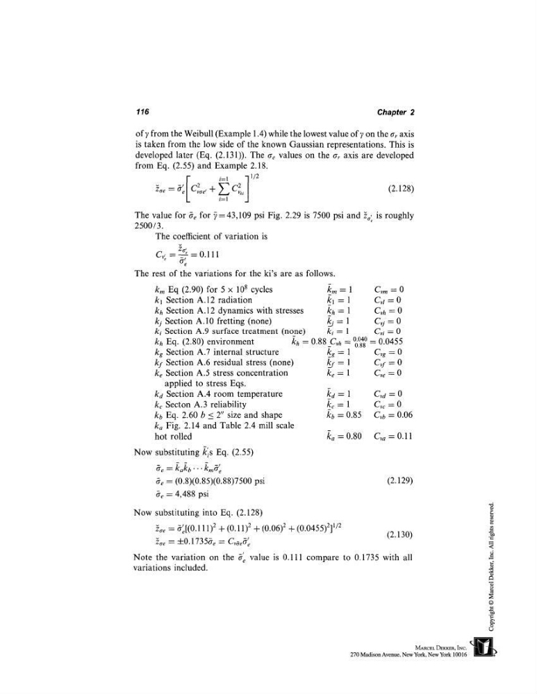
Ztre ": fie Cvae’ -l-The value for be for ~ ---- 43,109 psi Fig. 2.29 is 7500 psi andzo~V, is roughly
2500/3.
The coefficient of variation is
cg-Z<_, =0.111
O" e
The rest of the variations for the ki’s are as follows.
km Eq (2.90) for 5 x 10⁸ cycles
~m = 1
Cvm = 0
kl Section A.12 radiation
E 1 = 1
Cv~ = 0
kh Section A.12 dynamics with stresses
kh = 1
Cvh = 0
kj Section A. 10 fretting (none)
~ = 1
C~j = 0
ki Section A.9 surface treatment (no_ne)
ki = 1
Cvi = 0
Now
kh Eq. (2.80) environment
kh = 0.88 Cvh = °6!~48° = 0.0455
kg Section A.7 internal structure
~Cg = 1
Cvg = 0
kf Section A.6 residual stress (none)
~ = 1
Cvf = 0
ke Section A.5 stress concentration
ke = 1
Cve = 0
applied to stress Eqs.
ka Section A.4 room temperature
kc Secton A.3 reliability
kb Eq. 2.60 b < 2" size and shape
ka Fig. 2.14 and Table 2.4 mill scale
hot rolled
substituting ~:’,.s Eq. (2.55)
~e ~- kakb.., km~r
e
~e = (0.8)(0.85)(0.88)7500
6"e = 4,488 psi
1
Cvd = 0
~c=l
C~c=O
0.85
Cvb = 0.06
~a = 0.80 Cva = 0.11
(2.129)
Now substituting into Eq. (2.128)
-~re = 6"~e[(0.111) 2 q’- (0.11) 2 + (0.06) 2 -~ (0.0455)2]
U2
(2.130)
~e = d:0.17356e = Cv6e~’e
Note the variation on the a’e value is 0.111 compare to 0.1735 with all
variations included.
Chapter 2
of~ from the Weibull (Example 1.4) while the lowest value of~ on the O" r axis
is taken from the low side of the known Gaussian representations. This is
developed later (Eq. (2.131)). The O’e values on O- r axisare d eveloped
from Eq. (2.55) and Example 2.18.
I
i=1
I 1/2
~
-, 2
~ C
2
(2.128)
Ztre ": fie Cvae’ -l-The value for be for ~ ---- 43,109 psi Fig. 2.29 is 7500 psi andzo~V, is roughly
2500/3.
The coefficient of variation is
cg-Z<_, =0.111
O" e
The rest of the variations for the ki’s are as follows.
km Eq (2.90) for 5 x 10⁸ cycles
~m = 1
Cvm = 0
kl Section A.12 radiation
E 1 = 1
Cv~ = 0
kh Section A.12 dynamics with stresses
kh = 1
Cvh = 0
kj Section A. 10 fretting (none)
~ = 1
C~j = 0
ki Section A.9 surface treatment (no_ne)
ki = 1
Cvi = 0
Now
kh Eq. (2.80) environment
kh = 0.88 Cvh = °6!~48° = 0.0455
kg Section A.7 internal structure
~Cg = 1
Cvg = 0
kf Section A.6 residual stress (none)
~ = 1
Cvf = 0
ke Section A.5 stress concentration
ke = 1
Cve = 0
applied to stress Eqs.
ka Section A.4 room temperature
kc Secton A.3 reliability
kb Eq. 2.60 b < 2" size and shape
ka Fig. 2.14 and Table 2.4 mill scale
hot rolled
substituting ~:’,.s Eq. (2.55)
~e ~- kakb.., km~r
e
~e = (0.8)(0.85)(0.88)7500
6"e = 4,488 psi
1
Cvd = 0
~c=l
C~c=O
0.85
Cvb = 0.06
~a = 0.80 Cva = 0.11
(2.129)
Now substituting into Eq. (2.128)
-~re = 6"~e[(0.111) 2 q’- (0.11) 2 + (0.06) 2 -~ (0.0455)2]
U2
(2.130)
~e = d:0.17356e = Cv6e~’e
Note the variation on the a’e value is 0.111 compare to 0.1735 with all
variations included.