

67 Characteristics and Source Contribution of Particulate …
423
0.00
1.00
2.00
3.00
4.00
5.00
6.00
Jan-09 Jun-09 Dec-09 Jun-10 Dec-10 Jun-11 Dec-11 Jun-12 Dec-12 Jun-13 Dec-13 Jun-14 Dec-14
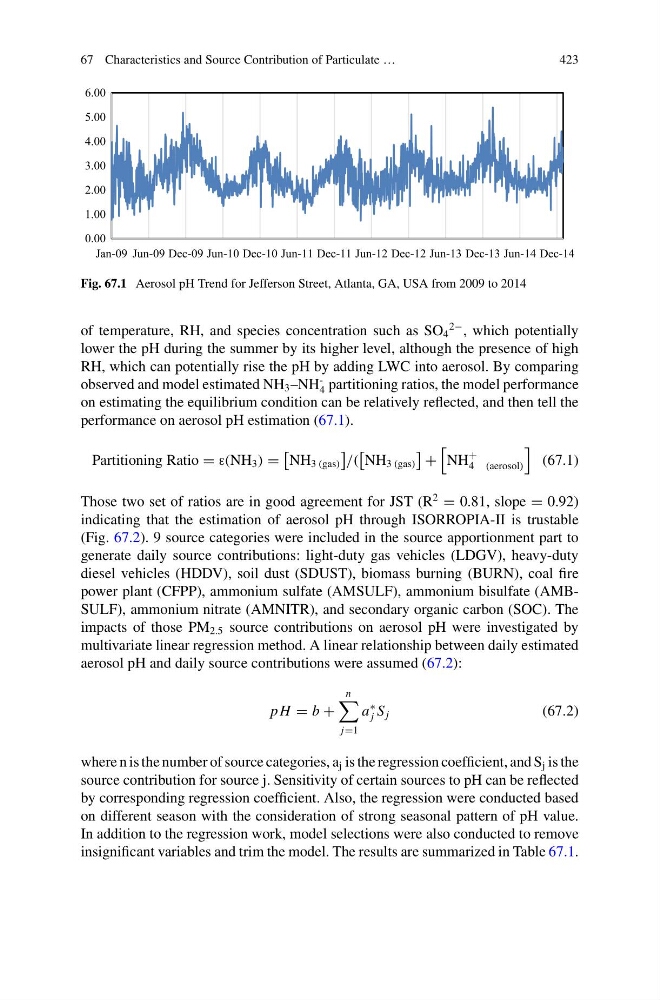
Fig. 67.1 Aerosol pH Trend for Jefferson Street, Atlanta, GA, USA from 2009 to 2014
of temperature, RH, and species concentration such as SO 4
2− , which potentially
lower the pH during the summer by its higher level, although the presence of high
RH, which can potentially rise the pH by adding LWC into aerosol. By comparing
observed and model estimated NH 3 –NH
-
4 partitioning ratios, the model performance
on estimating the equilibrium condition can be relatively reflected, and then tell the
performance on aerosol pH estimation (67.1).
Partitioning Ratio = ε(NH 3 ) =
NH 3 (gas)
/(
NH 3 (gas)
+
NH
+
4 (aerosol)
(67.1)
Those two set of ratios are in good agreement for JST (R
2
= 0.81, slope = 0.92)
indicating that the estimation of aerosol pH through ISORROPIA-II is trustable
(Fig. 67.2). 9 source categories were included in the source apportionment part to
generate daily source contributions: light-duty gas vehicles (LDGV), heavy-duty
diesel vehicles (HDDV), soil dust (SDUST), biomass burning (BURN), coal fire
power plant (CFPP), ammonium sulfate (AMSULF), ammonium bisulfate (AMBSULF), ammonium nitrate (AMNITR), and secondary organic carbon (SOC). The
impacts of those PM 2.5 source contributions on aerosol pH were investigated by
multivariate linear regression method. A linear relationship between daily estimated
aerosol pH and daily source contributions were assumed (67.2):
pH = b +
n
j=1
a
∗
j S j
(67.2)
where n is the number of source categories, a j is the regression coefficient, and S j is the
source contribution for source j. Sensitivity of certain sources to pH can be reflected
by corresponding regression coefficient. Also, the regression were conducted based
on different season with the consideration of strong seasonal pattern of pH value.
In addition to the regression work, model selections were also conducted to remove
insignificant variables and trim the model. The results are summarized in Table 67.1.
423
0.00
1.00
2.00
3.00
4.00
5.00
6.00
Jan-09 Jun-09 Dec-09 Jun-10 Dec-10 Jun-11 Dec-11 Jun-12 Dec-12 Jun-13 Dec-13 Jun-14 Dec-14
Fig. 67.1 Aerosol pH Trend for Jefferson Street, Atlanta, GA, USA from 2009 to 2014
of temperature, RH, and species concentration such as SO 4
2− , which potentially
lower the pH during the summer by its higher level, although the presence of high
RH, which can potentially rise the pH by adding LWC into aerosol. By comparing
observed and model estimated NH 3 –NH
-
4 partitioning ratios, the model performance
on estimating the equilibrium condition can be relatively reflected, and then tell the
performance on aerosol pH estimation (67.1).
Partitioning Ratio = ε(NH 3 ) =
NH 3 (gas)
/(
NH 3 (gas)
+
NH
+
4 (aerosol)
(67.1)
Those two set of ratios are in good agreement for JST (R
2
= 0.81, slope = 0.92)
indicating that the estimation of aerosol pH through ISORROPIA-II is trustable
(Fig. 67.2). 9 source categories were included in the source apportionment part to
generate daily source contributions: light-duty gas vehicles (LDGV), heavy-duty
diesel vehicles (HDDV), soil dust (SDUST), biomass burning (BURN), coal fire
power plant (CFPP), ammonium sulfate (AMSULF), ammonium bisulfate (AMBSULF), ammonium nitrate (AMNITR), and secondary organic carbon (SOC). The
impacts of those PM 2.5 source contributions on aerosol pH were investigated by
multivariate linear regression method. A linear relationship between daily estimated
aerosol pH and daily source contributions were assumed (67.2):
pH = b +
n
j=1
a
∗
j S j
(67.2)
where n is the number of source categories, a j is the regression coefficient, and S j is the
source contribution for source j. Sensitivity of certain sources to pH can be reflected
by corresponding regression coefficient. Also, the regression were conducted based
on different season with the consideration of strong seasonal pattern of pH value.
In addition to the regression work, model selections were also conducted to remove
insignificant variables and trim the model. The results are summarized in Table 67.1.