

330
S. Hanna and J. Chang
To assess dispersion model performance and uncertainties, the models are evaluated by comparison with several sets of field data. The BOOT model evaluation
software [2, 4] is widely used to evaluate the performance of individual models. The
software also allows the differences in the statistical performance measures between
several models to be assessed to determine whether they are significant at some
confidence level (usually 95%). The BOOT methodology for assessing confidence
limits is demonstrated here using several urban puff dispersion models applied to
the Oklahoma City Joint Urban 2003 (JU2003) field data [1, 3] as part of the Urban
Dispersion International Evaluation Exercise (UDINEE) [5].
A formal statistical test such as that in BOOT is needed to compare the performance measures for two models. BOOT automatically can account for the possibility
that the two models’ predictions may be correlated. For example, if the concentrations predicted by model B are always exactly two times those predicted by model A,
then there will always be a significant difference between the performance measures
calculated for the two models. This can be shown by expanding the formula for the
variance between fluctuations in two variables X and Y, and finding that a term “-2R”
is present, where R is the correlation between fluctuations in X and in Y.
52.2 Statistical Methods
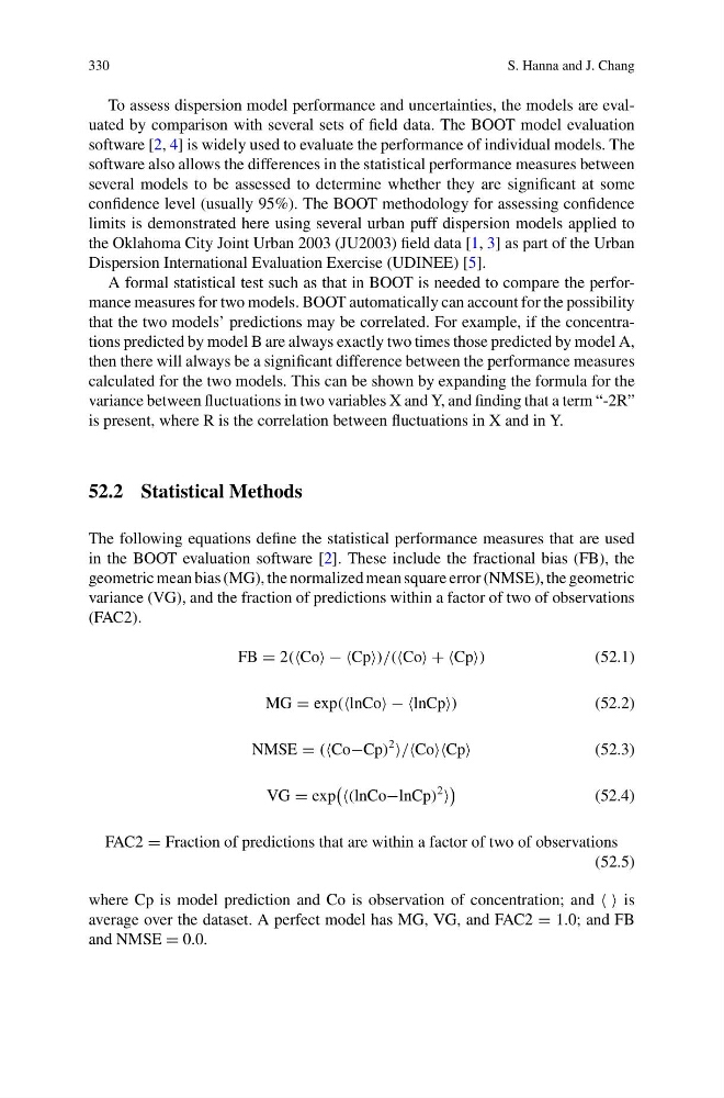
The following equations define the statistical performance measures that are used
in the BOOT evaluation software [2]. These include the fractional bias (FB), the
geometric mean bias (MG), the normalized mean square error (NMSE), the geometric
variance (VG), and the fraction of predictions within a factor of two of observations
(FAC2).
FB = 2(Co − −Cp)/(Co + +Cp)
(52.1)
MG = exp(lnCo − −lnCp)
(52.2)
NMSE = (Co−Cp)
2
/CoCp
(52.3)
VG = exp
(lnCo−lnCp)
2
(52.4)
FAC2 = Fraction of predictions that are within a factor of two of observations
(52.5)
where Cp is model prediction and Co is observation of concentration; and is
average over the dataset. A perfect model has MG, VG, and FAC2 = 1.0; and FB
and NMSE = 0.0.
S. Hanna and J. Chang
To assess dispersion model performance and uncertainties, the models are evaluated by comparison with several sets of field data. The BOOT model evaluation
software [2, 4] is widely used to evaluate the performance of individual models. The
software also allows the differences in the statistical performance measures between
several models to be assessed to determine whether they are significant at some
confidence level (usually 95%). The BOOT methodology for assessing confidence
limits is demonstrated here using several urban puff dispersion models applied to
the Oklahoma City Joint Urban 2003 (JU2003) field data [1, 3] as part of the Urban
Dispersion International Evaluation Exercise (UDINEE) [5].
A formal statistical test such as that in BOOT is needed to compare the performance measures for two models. BOOT automatically can account for the possibility
that the two models’ predictions may be correlated. For example, if the concentrations predicted by model B are always exactly two times those predicted by model A,
then there will always be a significant difference between the performance measures
calculated for the two models. This can be shown by expanding the formula for the
variance between fluctuations in two variables X and Y, and finding that a term “-2R”
is present, where R is the correlation between fluctuations in X and in Y.
52.2 Statistical Methods
The following equations define the statistical performance measures that are used
in the BOOT evaluation software [2]. These include the fractional bias (FB), the
geometric mean bias (MG), the normalized mean square error (NMSE), the geometric
variance (VG), and the fraction of predictions within a factor of two of observations
(FAC2).
FB = 2(Co − −Cp)/(Co + +Cp)
(52.1)
MG = exp(lnCo − −lnCp)
(52.2)
NMSE = (Co−Cp)
2
/CoCp
(52.3)
VG = exp
(lnCo−lnCp)
2
(52.4)
FAC2 = Fraction of predictions that are within a factor of two of observations
(52.5)
where Cp is model prediction and Co is observation of concentration; and is
average over the dataset. A perfect model has MG, VG, and FAC2 = 1.0; and FB
and NMSE = 0.0.