

240
R. Ménard and M. Deshaies-Jacques
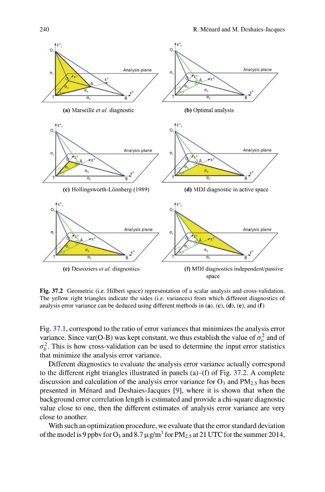
(a) Marseille et al. diagnostic
(b) Optimal analysis
(c) Hollingsworth-Lönnberg (1989)
(d) MDJ diagnostic in active space
(e) Desroziers et al. diagnostics
(f) MDJ diagnostics independent/passive
space
Fig. 37.2 Geometric (i.e. Hilbert space) representation of a scalar analysis and cross-validation.
The yellow right triangles indicate the sides (i.e. variances) from which different diagnostics of
analysis error variance can be deduced using different methods in (a), (c), (d), (e), and (f)
Fig. 37.1, correspond to the ratio of error variances that minimizes the analysis error
variance. Since var(O-B) was kept constant, we thus establish the value of σ
2
o and of
σ
2
b . This is how cross-validation can be used to determine the input error statistics
that minimize the analysis error variance.
Different diagnostics to evaluate the analysis error variance actually correspond
to the different right triangles illustrated in panels (a)–(f) of Fig. 37.2. A complete
discussion and calculation of the analysis error variance for O 3 and PM 2.5 has been
presented in Ménard and Deshaies-Jacques [9], where it is shown that when the
background error correlation length is estimated and provide a chi-square diagnostic
value close to one, then the different estimates of analysis error variance are very
close to another.
With such an optimization procedure, we evaluate that the error standard deviation
of the model is 9 ppbv for O 3 and 8.7 µg/m
3 for PM 2.5 at 21 UTC for the summer 2014,
R. Ménard and M. Deshaies-Jacques
(a) Marseille et al. diagnostic
(b) Optimal analysis
(c) Hollingsworth-Lönnberg (1989)
(d) MDJ diagnostic in active space
(e) Desroziers et al. diagnostics
(f) MDJ diagnostics independent/passive
space
Fig. 37.2 Geometric (i.e. Hilbert space) representation of a scalar analysis and cross-validation.
The yellow right triangles indicate the sides (i.e. variances) from which different diagnostics of
analysis error variance can be deduced using different methods in (a), (c), (d), (e), and (f)
Fig. 37.1, correspond to the ratio of error variances that minimizes the analysis error
variance. Since var(O-B) was kept constant, we thus establish the value of σ
2
o and of
σ
2
b . This is how cross-validation can be used to determine the input error statistics
that minimize the analysis error variance.
Different diagnostics to evaluate the analysis error variance actually correspond
to the different right triangles illustrated in panels (a)–(f) of Fig. 37.2. A complete
discussion and calculation of the analysis error variance for O 3 and PM 2.5 has been
presented in Ménard and Deshaies-Jacques [9], where it is shown that when the
background error correlation length is estimated and provide a chi-square diagnostic
value close to one, then the different estimates of analysis error variance are very
close to another.
With such an optimization procedure, we evaluate that the error standard deviation
of the model is 9 ppbv for O 3 and 8.7 µg/m
3 for PM 2.5 at 21 UTC for the summer 2014,