

196
V. Matthias et al.
30.3.2 Temporal Disaggregation
Most of the emission inventories provide only annual values, however, some contain
seasonal variations with monthly emission maps (e.g. HTAP2.2 [9], ECLIPSE [10]
or REAS 2.1 [14]). For model ready emission data, the temporal variation of specific
source sectors is considered via the application of typical time profiles. They are
typically divided into fixed monthly, weekly and daily variations with no dependence
on season or location.
However, the spatial and temporal allocation of emissions can be improved, as
some publications demonstrated for ammonia [2, 6, 17]. Skjoth et al. [17] and Backes
et al. [2] proposed to split emissions from agriculture into animal husbandry, manure
management and fertilizer use. Emissions from stables can be modelled according
to ambient temperatures and wind velocity, manure management needs to follow
legislative restrictions and fertilizer use depends on season and crop growing times.
A similar approach was followed by Hendricks et al. [6] for agricultural emissions
in the Netherlands.
Menut et al. [12] investigated diurnal cycles of traffic emissions in several European cities. They found significant differences between northern European cities and
those in the South and considered this in their regional scale chemistry transport
model calculations with the CHIMERE model. Mues et al. [13] followed a similar approach for traffic emissions in Germany. Both studies revealed similar results.
While correlation coefficients for NO 2 , O 3 and PM 2.5 were improved when the model
results were compared to observations, the mean concentrations showed only small
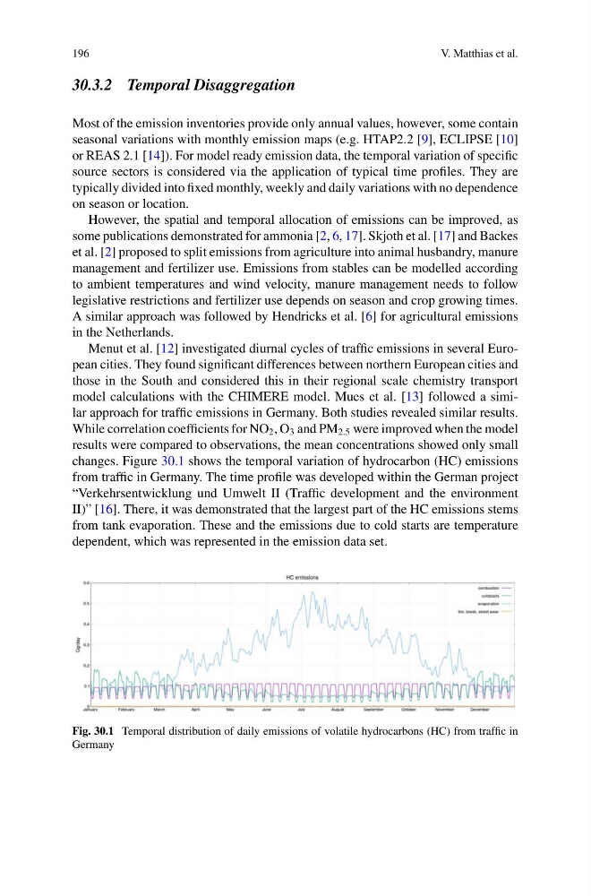
changes. Figure 30.1 shows the temporal variation of hydrocarbon (HC) emissions
from traffic in Germany. The time profile was developed within the German project
“Verkehrsentwicklung und Umwelt II (Traffic development and the environment
II)” [16]. There, it was demonstrated that the largest part of the HC emissions stems
from tank evaporation. These and the emissions due to cold starts are temperature
dependent, which was represented in the emission data set.
Fig. 30.1 Temporal distribution of daily emissions of volatile hydrocarbons (HC) from traffic in
Germany
V. Matthias et al.
30.3.2 Temporal Disaggregation
Most of the emission inventories provide only annual values, however, some contain
seasonal variations with monthly emission maps (e.g. HTAP2.2 [9], ECLIPSE [10]
or REAS 2.1 [14]). For model ready emission data, the temporal variation of specific
source sectors is considered via the application of typical time profiles. They are
typically divided into fixed monthly, weekly and daily variations with no dependence
on season or location.
However, the spatial and temporal allocation of emissions can be improved, as
some publications demonstrated for ammonia [2, 6, 17]. Skjoth et al. [17] and Backes
et al. [2] proposed to split emissions from agriculture into animal husbandry, manure
management and fertilizer use. Emissions from stables can be modelled according
to ambient temperatures and wind velocity, manure management needs to follow
legislative restrictions and fertilizer use depends on season and crop growing times.
A similar approach was followed by Hendricks et al. [6] for agricultural emissions
in the Netherlands.
Menut et al. [12] investigated diurnal cycles of traffic emissions in several European cities. They found significant differences between northern European cities and
those in the South and considered this in their regional scale chemistry transport
model calculations with the CHIMERE model. Mues et al. [13] followed a similar approach for traffic emissions in Germany. Both studies revealed similar results.
While correlation coefficients for NO 2 , O 3 and PM 2.5 were improved when the model
results were compared to observations, the mean concentrations showed only small
changes. Figure 30.1 shows the temporal variation of hydrocarbon (HC) emissions
from traffic in Germany. The time profile was developed within the German project
“Verkehrsentwicklung und Umwelt II (Traffic development and the environment
II)” [16]. There, it was demonstrated that the largest part of the HC emissions stems
from tank evaporation. These and the emissions due to cold starts are temperature
dependent, which was represented in the emission data set.
Fig. 30.1 Temporal distribution of daily emissions of volatile hydrocarbons (HC) from traffic in
Germany