

422
32 On Boundary Value Problems of Inelastic Body Mechanics
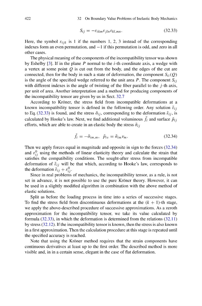
S ij = −ε ikm ε jln ε kl,mn .
(32.33)
Here, the symbol ε ij k is 1 if the numbers 1, 2, 3 instead of the corresponding
indexes form an even permutation, and −1 if this permutation is odd, and zero in all
other cases.
The physical meaning of the components of the incompatibility tensor was shown
by Eshelby [3]. If in the plane P normal to the i-th coordinate axis, a wedge with
a vertex at some point Q is cut out from the body, and the edges of the cut are
connected, then for the body in such a state of deformation, the component S ii (Q)
is the angle of the specified wedge referred to the unit area P . The component S ij
with different indexes is the angle of twisting of the fiber parallel to the j -th axis,
per unit of area. Another interpretation and a method for producing components of
the incompatibility tensor are given by us in Sect. 32.7
According to Kröner, the stress field from incompatible deformations at a
known incompatibility tensor is defined in the following order. Any solution ˜
ε ij
to Eq. (32.33) is found, and the stress ˜
σ ij , corresponding to the deformation ˜
ε ij , is
calculated by Hooke’s law. Next, we find additional voluminous ˜
f i and surface ˜
p ij
efforts, which are able to create in an elastic body the stress ˜
σ ij
˜
f i = − ˜
σ im,m , ˜
p iν = ˜
σ im ν m .
(32.34)
Then we apply forces equal in magnitude and opposite in sign to the forces (32.34)
and ε 0
ij using the methods of linear elasticity theory and calculate the strain that
satisfies the compatibility conditions. The sought-after stress from incompatible
deformation of ˜
ε ij will be that which, according to Hooke’s law, corresponds to
the deformation ˜
ε ij + ε 0
ij .
Since in real problems of mechanics, the incompatibility tensor, as a rule, is not
set in advance, it is not possible to use the pure Kröner theory. However, it can
be used in a slightly modified algorithm in combination with the above method of
elastic solutions.
Split as before the loading process in time into a series of successive stages.
To find the stress field from discontinuous deformations at the (k + 1)-th stage,
we apply the above-described procedure of successive approximations. As a zeroth
approximation for the incompatibility tensor, we take its value calculated by
formula (32.33), in which the deformation is determined from the relations (32.11)
by stress (32.12). If the incompatibility tensor is known, then the stress is also known
in a first approximation. Then the calculation procedure at this stage is repeated until
the specified accuracy is reached.
Note that using the Kröner method requires that the strain components have
continuous derivatives at least up to the first order. The described method is more
visible and, in in a certain sense, elegant in the case of flat deformation.
32 On Boundary Value Problems of Inelastic Body Mechanics
S ij = −ε ikm ε jln ε kl,mn .
(32.33)
Here, the symbol ε ij k is 1 if the numbers 1, 2, 3 instead of the corresponding
indexes form an even permutation, and −1 if this permutation is odd, and zero in all
other cases.
The physical meaning of the components of the incompatibility tensor was shown
by Eshelby [3]. If in the plane P normal to the i-th coordinate axis, a wedge with
a vertex at some point Q is cut out from the body, and the edges of the cut are
connected, then for the body in such a state of deformation, the component S ii (Q)
is the angle of the specified wedge referred to the unit area P . The component S ij
with different indexes is the angle of twisting of the fiber parallel to the j -th axis,
per unit of area. Another interpretation and a method for producing components of
the incompatibility tensor are given by us in Sect. 32.7
According to Kröner, the stress field from incompatible deformations at a
known incompatibility tensor is defined in the following order. Any solution ˜
ε ij
to Eq. (32.33) is found, and the stress ˜
σ ij , corresponding to the deformation ˜
ε ij , is
calculated by Hooke’s law. Next, we find additional voluminous ˜
f i and surface ˜
p ij
efforts, which are able to create in an elastic body the stress ˜
σ ij
˜
f i = − ˜
σ im,m , ˜
p iν = ˜
σ im ν m .
(32.34)
Then we apply forces equal in magnitude and opposite in sign to the forces (32.34)
and ε 0
ij using the methods of linear elasticity theory and calculate the strain that
satisfies the compatibility conditions. The sought-after stress from incompatible
deformation of ˜
ε ij will be that which, according to Hooke’s law, corresponds to
the deformation ˜
ε ij + ε 0
ij .
Since in real problems of mechanics, the incompatibility tensor, as a rule, is not
set in advance, it is not possible to use the pure Kröner theory. However, it can
be used in a slightly modified algorithm in combination with the above method of
elastic solutions.
Split as before the loading process in time into a series of successive stages.
To find the stress field from discontinuous deformations at the (k + 1)-th stage,
we apply the above-described procedure of successive approximations. As a zeroth
approximation for the incompatibility tensor, we take its value calculated by
formula (32.33), in which the deformation is determined from the relations (32.11)
by stress (32.12). If the incompatibility tensor is known, then the stress is also known
in a first approximation. Then the calculation procedure at this stage is repeated until
the specified accuracy is reached.
Note that using the Kröner method requires that the strain components have
continuous derivatives at least up to the first order. The described method is more
visible and, in in a certain sense, elegant in the case of flat deformation.