

19.2 Two-Dimensional Klyushnikov Model
289
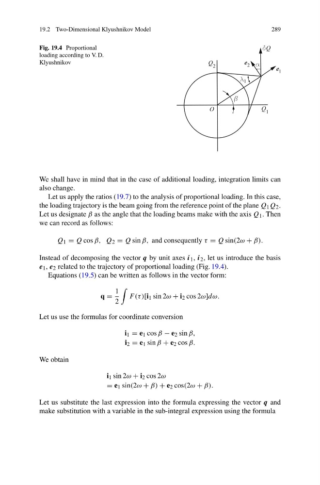
Fig. 19.4 Proportional
loading according to V. D.
Klyushnikov
We shall have in mind that in the case of additional loading, integration limits can
also change.
Let us apply the ratios (19.7) to the analysis of proportional loading. In this case,
the loading trajectory is the beam going from the reference point of the plane Q 1 Q 2 .
Let us designate β as the angle that the loading beams make with the axis Q 1 . Then
we can record as follows:
Q 1 = Q cos β, Q 2 = Q sin β, and consequently τ = Q sin(2ω + β).
Instead of decomposing the vector q by unit axes i 1 , i 2 , let us introduce the basis
e 1 , e 2 related to the trajectory of proportional loading (Fig. 19.4).
Equations (19.5) can be written as follows in the vector form:
q =
1
2
F (τ )[i 1 sin 2ω + i 2 cos 2ω]dω.
Let us use the formulas for coordinate conversion
i 1 = e 1 cos β − e 2 sin β,
i 2 = e 1 sin β + e 2 cos β.
We obtain
i 1 sin 2ω + i 2 cos 2ω
= e 1 sin(2ω + β) + e 2 cos(2ω + β).
Let us substitute the last expression into the formula expressing the vector q and
make substitution with a variable in the sub-integral expression using the formula
289
Fig. 19.4 Proportional
loading according to V. D.
Klyushnikov
We shall have in mind that in the case of additional loading, integration limits can
also change.
Let us apply the ratios (19.7) to the analysis of proportional loading. In this case,
the loading trajectory is the beam going from the reference point of the plane Q 1 Q 2 .
Let us designate β as the angle that the loading beams make with the axis Q 1 . Then
we can record as follows:
Q 1 = Q cos β, Q 2 = Q sin β, and consequently τ = Q sin(2ω + β).
Instead of decomposing the vector q by unit axes i 1 , i 2 , let us introduce the basis
e 1 , e 2 related to the trajectory of proportional loading (Fig. 19.4).
Equations (19.5) can be written as follows in the vector form:
q =
1
2
F (τ )[i 1 sin 2ω + i 2 cos 2ω]dω.
Let us use the formulas for coordinate conversion
i 1 = e 1 cos β − e 2 sin β,
i 2 = e 1 sin β + e 2 cos β.
We obtain
i 1 sin 2ω + i 2 cos 2ω
= e 1 sin(2ω + β) + e 2 cos(2ω + β).
Let us substitute the last expression into the formula expressing the vector q and
make substitution with a variable in the sub-integral expression using the formula